Four-Dimensional Object-Space Data Reconstruction Using Spatial-Spectral Multiplexing.

(1)

ABSTRACT

WU, ZHEJUN. Four-Dimensional Object-Space Data Reconstruction Using Spatial-Spectral Multiplexing. (Under the direction of Michael Kudenov.)

This thesis investigates the data reconstruction problem of a four-dimensional scene based on the Spatial-Spectral Multiplexing (SSM) technique. The SSM technique is used in a

hyper-spectral imaging system for the application of passive remote sensing. The thesis first introduces

the current development of the remote sensing field and its associated applications. The SSM technique, in particular, provides unique advantages over other systems in use for developing

longitudinal spatial coherence holograms because it can enable snapshot measurements of a

coherence function. Additionally, this technique can enable access to interference patterns that can be decomposed to access the phase information that is present (but inaccessible) in the

pupil of a conventional lens. Finally, due to this phase-sensitivity, the technique can also enable

an alternative interference-based method for passively sensing distance without the need for stereoscopic co-boresighted objectives or active illuminators. In this thesis, the concept is

ap-plied to the field of hyperspectral imaging because it can serve as a feasible problem to ascertain

methods of data reduction and reconstruction. Since the algorithm is based on the SSM system, the thesis illustrates its optical model and its related modulation model. Such a model yields a

challenging data reconstruction problem.

The goal of data reconstruction in the context of SSM and hyperspectral imaging is to use measurements from a given measurement matrix to recover the scene’s object locations

and object spectra. This can be formulated as an underdetermined linear system, thereby

producing an infinite number of potential solutions. The research work in this thesis proposes to solve the inverse problem by incorporating several heuristic prior assumptions and formulate

an optimization from a probabilistic perspective. Based on this notion, this thesis proposes

two categories of reconstruction methods: non-parametric and parametric. In particular, the thesis shows that by incorporating B-splines to reparameterize the object spectra, the number

of unknown variables is highly reduced in the linear system, so it can achieve a much more

accurate and efficient reconstruction for large scale data.

In order to validate the algorithm, three kinds of synthetic ground truth scene objects are

generated, with which the modulation model can simulate the measurements and the mea-surement matrix based on the SSM technique. To demonstrate the accuracy and efficiency of

this algorithm, the thesis compares the non-parametric method and parametric method based

on several reparameterization methods at various data scale. Besides, the Poisson noise with different SNRs is also added onto the measurements before optimization in order to test the

(2)

on both smoothly varying and point cloud objects for the SSM system. It can achieve a 0.2%

overall MSE without noise, and 0.3% overall MSE with noise (SNR greater than 30). The al-gorithm can handle a quite large data scale with the reparameterization method. The results

of this thesis show the potential of applying such reconstruction methods on real-life scenes in

(3)

(4)

Four-Dimensional Object-Space Data Reconstruction Using Spatial-Spectral Multiplexing

by Zhejun Wu

A thesis submitted to the Graduate Faculty of North Carolina State University

in partial fulfillment of the requirements for the Degree of

Master of Science

Electrical Engineering

Raleigh, North Carolina

2017

APPROVED BY:

Michael Escuti Edgar Lobaton

(5)

BIOGRAPHY

Zhejun Wu was born and grew up in Shanghai, an eastern coastal city of China. In her path of learning, she has cultivated great interests in science and engineering since her high school.

She majored in Electrical and Electronics Engineering as an undergraduate student in Shanghai Jiao Tong University, where she also completed her first master’s degree majoring in Instrument

Science and Engineering. After that she came to North Carolina State University to pursue her

second master’s degree, majoring in Electrical Engineering. During her study in NCSU, she was also an research assistant in the Optical Sensing Lab, under the advisement of Dr. Michael

(6)

TABLE OF CONTENTS

LIST OF FIGURES . . . iv

Chapter 1 Introduction . . . 1

1.1 Background . . . 1

1.1.1 Development in the remote sensing field . . . 1

1.1.2 The SSM technique . . . 3

1.1.3 Optical model of SSM systems . . . 3

1.2 Four-dimensional scene reconstruction using SSM . . . 5

1.3 Methodological design of the reconstruction algorithm . . . 6

1.4 Overview of chapters . . . 6

Chapter 2 Experimental materials and setup . . . 8

2.1 Three-dimensional piecewise spiral curves . . . 8

2.2 Multiple random points . . . 9

2.3 A specific scene . . . 12

2.4 Experimental setup . . . 12

2.5 Conclusion . . . 14

Chapter 3 Non-parametric data reconstruction . . . 15

3.1 Posterior optimization for an underdetermined linear system . . . 15

3.1.1 Heuristic prior assumptions . . . 16

3.1.2 Likelihood . . . 17

3.1.3 MAP analysis . . . 18

3.2 The L-BFGS numerical method . . . 19

3.3 Reconstruction results . . . 19

Chapter 4 Parametric data reconstruction . . . 30

4.1 The RKHS reparameterization model . . . 31

4.2 The B-spline reparameterization model . . . 33

4.3 Reconstruction results . . . 35

Chapter 5 Conclusion and discussion . . . 47

(7)

LIST OF FIGURES

Figure 1.1 Two dimensional modulation model . . . 4

Figure 2.1 3D-spatial piecewise spiral object . . . 10 Figure 2.2 Spectral intensity functions sampled from a Gaussian Process . . . 11 Figure 2.3 Cross-sectional planes of the ground truth object with 100 random points . . 12 Figure 2.4 Specific scene of three bars shown by point clouds . . . 13

Figure 3.1 The ground truth for the spiral curves object . . . 21 Figure 3.2 Reconstruction results for the low resolution spiral curves object without

using any prior assumptions . . . 22 Figure 3.3 Reconstruction results for the low resolution spiral curves object using the

non-parametric method with the spatial smoothness assumption . . . 23 Figure 3.4 Reconstruction results for the low resolution spiral curves object using the

non-parametric method with the spectral smoothness assumption . . . 24 Figure 3.5 Reconstruction results for the low resolution spiral curves object using the

non-parametric method with both spatial and spectral smoothness assumptions 25 Figure 3.6 Reconstruction results for the spiral curves object using the non-parametric

method with both spatial and spectral smoothness assumptions . . . 26 Figure 3.7 The ground truth for the random point cloud object . . . 28 Figure 3.8 Reconstruction results for the random point cloud object using the

non-parametric method with the spectral smoothness assumption . . . 29

Figure 4.1 A linear function is projected onto the first 1000 eigenfunctions. The projec-tion coefficients are shown in the above figure. . . 32 Figure 4.2 B-spline functions with order 4 and 10 knots . . . 34 Figure 4.3 Reconstruction results for spiral curves object using the RHKS parametric

method . . . 36 Figure 4.4 Reconstruction results for spiral curves object using the B-spline parametric

method . . . 38 Figure 4.5 Reconstruction results for the random point cloud object using the B-spline

parametric method . . . 39 Figure 4.6 The ground truth for the 3-bar object . . . 40 Figure 4.7 Reconstruction results for the 3-bar object using the B-spline parametric

method . . . 41 Figure 4.8 The spectral intensity of 3-bar ground truth and reconstructed results using

the B-spline parametric method . . . 42 Figure 4.9 Reconstruction results for the 3-bar object using the B-spline parametric

method with Poisson noise . . . 43 Figure 4.10 The overal MSEs of recovering three objects from noised measurements with

different SNR using the B-spline parametric method . . . 44 Figure 4.11 The time costs of recovering object with different data scales using the

(8)

(9)

Chapter 1

Introduction

This section will first introduce the development, applications and current limitations of the remote sensing. Then it will analyze some hyperspectral imaging techniques that are widely

used to improve remote sensing technology, and will also propose a Spatial-Spectral

Multiplex-ing (SSM) technique, which can be used in hyperspectral imagMultiplex-ing. Based on these theoretical backgrounds, the section will introduce the modulation model of the SSM system, which is

also the optical model for this reconstruction algorithm. After that, it will briefly describe the

research purpose and give an outline of the proposed methods. Additionally, an overview of the following content will be presented in the end of this chapter.

1.1 Background

1.1.1 Development in the remote sensing field

The term ”remote sensing” was first used in 1960s by a scientist of U.S. Navy’s Office of Navals

Research[4]. There are various definitions for remote sensing. Generally speaking, remote sensing

is a scientific technology of acquiring information from an object, an area or any phenomenon and analyzing the acquired data[17]. The devices or sensor systems used to obtain these useful

data are not directly in contact with the objects need to be identified or measured[20].

It has been well-known that the sensors could be divided into active and passive based on the source of energy. Remote sensing that relies on solar and terrestrial energy belongs to

the passive sensor systems. Taking the example of the solar energy, which accounts for the

vast majority of the non-human-made sources, the sunlight is reflected, emitted or transmitted from the objects and recorded by the passive devices. There are also remote sensing systems

working with active sensors[15], which emit the energy sources such as radar, sonar and laser by

(10)

categories: (1) visible and reflective infrared, (2) thermal infrared and (3) microwave remote

sensing[14]. The former two types are passively detected, while the microwave type can be based on either passive or active sensors. The algorithms and techniques provided in this thesis are

aimed to be applied for passive, visible and reflective infrared remote sensing.

One of the most straightforward passive sensors for remote sensing are eyes[10]. Human beings have been eager to know about the earth and space since a long time ago. Not limited to

their eyes, humans began to make use of external tools, such as telescopes, to visualize the area

outside the field of view. The invention of photography was another milestone in the history of remote sensing. Using the photography technology, humans tried to observe the ground and

take photographs at a greater height on the mountain or in a balloon. During this initial period,

remote sensing were still referred as aerial photography[22]. Afterwards, the technique of aerial photography steadily evolved due to the improvement in platforms, camera hardwares and

photo interpolation techniques. The rapid growing of interests in remote sensing started after

the successful launch of artificial satellites. To date, there are three main platforms in remote sensing: ground-based, airborne and space borne[14]. As the name implies, they are classified

by the height from the earth’s surface. The remote sensors are mounted on these platforms to

detect the electromagnetic energy reflected from the earth’s surface, which can be mapped to the prior knowledge of some features[16]. Multispectral images are one of the most common

images acquired by the remote sensors. In recent years, further improvement in sensors and satellites has greatly increased the quality of data and the accuracy of mapping by providing

us not only multispectral images but also hyperspectral images[25].

Remote sensing has played an increasingly vital role in numerous applications fields. These include crop monitoring and type classification in the field of agriculture; flood, landslides and

volcanic activity observation; geological structure mapping and natural resources exploration.

There are also many promising applications in the field of hydrology, oceanography, glaciology, forest, climate, urban, military and meteorology[11]. With remotely sensed images and data,

human beings have widely broadened the field of view and range of cognition.

These applications, however, can still be limited by the quality of image data, especially the image resolution and sampling frequency. There are some important properties of the remote

sensing data: spatial resolution/sampling, radiometric resolution, spectral resolution/sampling

and temporal resolution/sampling. The resolution means the maximum discrimination of a measurement, and the sampling refers to the sample frequency to collect the data. This thesis

will mainly focus on the spatial and spectral resolution/sampling, where the spectral resolution

(11)

1.1.2 The SSM technique

In order to surpass the limit of image quality, some new imaging techniques have been proposed

to acquire a higher spectral resolution and a larger spatial coverage for remote sensing. For

example, the multispectral imaging makes it possible to obtain the spectral features of many bands simultaneously[24]; hyperspectral imaging[7] makes it possible to acquire continuous and

complete spectral information of each spatial location across the scene[27]. The most important

part of these imaging spectroscopy methods are the imaging sensors have very high spectral resolution. Using such hyperspectral imaging techniques, a conventional way to obtain the

three-dimensional(3D) spatial and spectral information of a scene is to use temporal scanning to scan

the entire scene with a two-dimensional(2D) sensor. However, this method can only be applied on static objects[18]. Other non-scanning methods, such as the snapshot approach, have also

achieved major advances. Snapshot spectral imaging can record a 3D object-space datacube by multiplexing the high-dimensional signal onto the 2D sensor[28].

With the same motivation, the SSM theory was also presented in [29]. The pivotal idea

behind the SSM technique is that it can encode angular information of a scene onto the incident power spectrum. To be specific, the SSM technique uses the two-beam interference, generated

from a spectrally-resolved interferometer, to represent every object point and to modulate the

angular spectrum (incident angle) of each object point onto a spectral carrier frequency using the Fourier basis function. This means that the resultant channeled spectrum contains both

phase and amplitude information, such that the spatial and spectral content of the scene can

be reconstructed. Additionally, the SSM technique enables phase retrieval to be achieved from the pupil of an imaging system, without the use of a lens. Based on this SSM technique, the

spatial-spectral multiplexer can be agnostic, and includes interferometers such as Fabry Perot

Etalon (FPE), Michelson Interferometer (MI), MachZehnder (MZ) interferometer, etc.

Compared with the other state-of-the-art hyperspectral imaging techniques, the advantages

of SSM are: first, it can encode four-dimensional(4D) scene information using 3D spectrometer

measurements, which can reduce the amount of data needed during the measurement. Second, the SSM technique uses a 3D spectrometer array to sample the pupil of the spatial-spectral

modulator, so that we do not need to form images before reconstruction, which provides a

more computational imaging process. The limitation of SSM is that it has not achieved much improvement in the spatial resolution in hyperspectral imaging.

1.1.3 Optical model of SSM systems

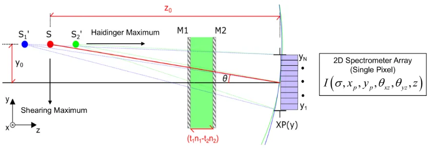
The measurements of SSM systems are simulated through modulation. The 2D modulation is needed to encode the object information onto the 2D spectrometer array for a 4D object-space

(12)

because the system only need a 1D spectrometer array to sample the pupil. Since the SSM

tech-nique uses two-beam interference to modulate the spatial information onto the power spectrum, there are two point sources for each spatial location of the object in this model. As shown in

Figure 1.1, the red spot is one of the actual object sampling points. The blue and green ones

are the two simulated point sources. Figure 1.1 illustrates the modulation process for each of they−z planes in the 2D case.

Figure 1.1: Two dimensional modulation model

The 4D object is in the space of the Cartesian product of the 3D spatial domain and

the 1D spectral domain, which can be expressed by a 4D function f(σ, θxz, θyz, z). Here, σ

is the wavenumber, θxz and θyz are the incident angles in x−z and y−z planes, and z is

the distance from the object sampling point to the pupil plane in z direction. For notational

simplicity, the following thesis will also usef to denote the 4D object functionf(σ, θxz, θyz, z).

The measurement with the 2D-spatial pupil plane g(σ, xp, yp) is simulated by the dot product

between the measurement matrixH and objectf, as shown in Eq. 1.1.

g(σ, xi_p, yj_p) =

N X n=1 M X m=1 K X k=1

H(σ, xi_p, yj_p, θn_xz, θ_yzm, zk)·f(σ, θn_xz, θm_yz, zk), (1.1)

wherei,j,m,nand kare the indexes of the variables. Assuming a perfect spherical wave, the channeled spectrumH(σ, xi

p, y j

p, θnxz, θyzm, zk) is computed as follow:

H(σ, xi_p, y_pj, θn_xz, θm_yz, zk) = 1

(13)

spectrum. Therefore, the measurement matrix H is made of the channeled spectra between

each object point and each detector location. In Eq. 1.2,r1 and r2 are the distances from the

two object point sources to the spectrometer, which can be computed by

r1 =

q ((xi

p−zk·tan(θnxz))2+ ((y j

p−zk·tan(θyzm)2+ (zk−OPD(σ/2))2, (1.3)

r2 =

q ((xi

p−zk·tan(θnxz))2+ ((y j

p−zk·tan(θyzm)2+ (zk+ OPD(σ/2))2. (1.4)

Here the Optical Path Difference (OPD) has either a positive sign or a negative sign depending on which one of the two point sources is being measured. Note that the OPD can be defined

differently according to the specific spatial-spectral multiplexer to be used. Details of this SSM

model can also be found in [29]. Such a model motivates the need of object reconstruction; that is, given the simulated measurementsg and the measurement matrixH, the goal is to estimate

the object f.

This Eq. 1.1 is essentially a linear equation. However, the number of pupil planes is smaller than the number of sources. Therefore the SSM system is an underdetermined linear system,

which means the algorithm do not have enough information to uniquely solve for the spectrum

of the object f. Therefore, to optimally recover f, some additional appropriate assumptions need to be incorporated into the object scenes. These assumptions will be further described in

Sec. 3.1.1.

1.2 Four-dimensional scene reconstruction using SSM

This section illustrates the problem going to be worked on and the research purpose. As

in-troduced in the background section, remote sensing relies on images with very fine spatial and spectral resolutions. The hyperspectral imaging is a widely used and rapidly growing imaging

technique in the remote sensing field. The problem needs to be solved is to develop an

recon-struction algorithm for an optical system using a new SSM hyperspectral imaging technique. Different from other hyperspectral imaging methods, the SSM system provides a more

com-putational way to obtain the spatial and spectral information of a scene and stores much less

amount of measurements. The method that the SSM technique uses to acquire the image infor-mation is computational imaging as it encodes the scene inforinfor-mation onto a 2D spectrometer

array, which is used to sample the pupil plane. The idea is that instead of producing complete sub-images with the same level of spatial dimensions as the object, the SSM system only needs

to record the multiplexed information with the same dimensions as the detector plane.

(14)

planes. The 4D object-space data can be a specific scene with 3D-spatial and 1D-spectral

infor-mation, as what we can perceived from the world around us. In the experiments, the scenes are indicated by point clouds. The requirements of this reconstruction algorithm are: (a) to work

on different realistic objects, including extended, random points and point clouds sources; (b)

to deal with relative large data sets (roughly 15 Gigabytes) within an acceptable running time; (c) to achieve high accuracy in cases of both with and without Poisson noise.

1.3 Methodological design of the reconstruction algorithm

This section gives an outline of the methodologies. There are two main challenges in the

re-construction algorithm: (a) since the SSM system only stores a small amount of multiplexed

information, the object from a highly underdetermined linear system (the number of unknown variables is larger than the number of linear equations) needs to be recovered, and a direct

psuedo-inverse will produce meaningless results; (b) the size of the 4D object is extremely

large. A non-parametric representation of the object will lead to a large-scale linear system that is numerically difficult to solve. In the experiments, a simple 1000×10×10×10 object

with a non-parametric representation will cost 100 Megabytes storage, and the reconstruction

can be extremely time consuming.

To handle the first challenge, the algorithm proposes several heuristic prior assumptions

that can adapt to the realistic 4D scenes, and with these priors the algorithm can uniquely

recover the object. Moreover, an optimization model is constructed to minimize the least square reconstruction error with the constraints of the aforementioned heuristic assumptions. To deal

with this second challenge, the algorithm proposes to reparameterize the 4D object data with

certain basis functions to reduce the number of unknown variables in the linear system. Several parametric models based on the eigenfunctions of Gaussian kernels and basis splines are tested

and compared. Additionally, a memory-efficient numerical method is also applied to accelerate

the optimization process.

1.4 Overview of chapters

After having an general idea of the background and its associated application, the following four chapters of this thesis will describe the technical details of the reconstruction algorithm.

Chapter 2 will give the experiments materials, parameter settings of the SSM model and

de-scribe the experimental setup to test the reconstruction accuracy. The object models for the reconstruction tests include: 3D-spatial piecewise-smooth spiral curves, multiple random points

and a 3-bar scene model. Besides, the experimental setup for measuring the effect of Poisson

(15)

focused on the non-parametric data reconstruction method. It will introduce the specific

defini-tion of the realistic assumpdefini-tions on the objects and will also propose the optimizadefini-tion model for the linear system. Afterwards, Chapter 4 will elaborate on the parametric data reconstruction

method. It covers two reparameterization models and the comparison of their characteristics

and performances. Sec. 4.3 will compare the above two main data reconstruction methods, analyze the accuracy and computational efficiency as well as the robustness of the algorithm.

Finally, Chapter 5 will conclude the work and contributions of this thesis, as well as discuss

(16)

Chapter 2

Experimental materials and setup

Before giving the technical details of the proposed reconstruction methods, this chapter demon-strates the experimental materials and the parameter settings of the SSM model. In this work,

the experimental materials for validating the reconstruction algorithms are several synthetic

scenes. The main reason for using synthetic scenes in the experiment is that the use of SSM systems, including the optical model and the reconstruction methods, is still in its preliminary

stage. With the manually constructed ground truth objects in synthetic scenes, I can exactly

validate the reconstruction algorithm and draw insights from the results. Therefore, a common experimental setup is to first construct a ground truth synthetic scene (a synthetic objectf) and

to use the SSM optical model to produce its measurements in the detector. Finally, the object

will be reconstructed, denoted as f∗, from the measurements and compare the reconstructed object f∗ with the ground truth objectf to validate the reconstruction algorithm’s accuracy.

Three kinds of objects will be designed to be recovered by the reconstruction algorithm.

In order to test the generality of the algorithm, these objects have very different properties. To test the algorithm robustness, the noise will be added to the measurements before the

reconstruction. Sec. 2.4 will describe the adding noise procedure and the associated experiment

setup in detail.

2.1 Three-dimensional piecewise spiral curves

The first type of synthetic object is a 3D-spatial spiral curve, which is generated from the following steps:

(a) Construct a spiral curve in the 3D-spatial space;

(b) Randomly break the spiral curve into four intervals; (c) Randomly set different radii to the four spiral pieces;

(17)

(e) Smooth the object using a 3D Gaussian filter.

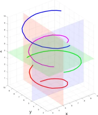
In this way, it becomes spatially smoothed 3D spiral curves with some random radii. Fig-ure 2.1 (a) shows the piecewise spiral curve object, where x and y donates the θxz and θyz

dimension of the objectf(σ, θxz, θyz, z) in Eq. 1.1. The corresponding 3D datacube is then

gen-erated and Figure 2.1 (b) shows three 2D cross-sectional slices. Each cross-sectional plane in Figure 2.1 (b) is labeled as a corresponding color as in the Figure 2.1 (a).

Due to the way of constructing the curve and the 3D Gaussian smoothing, the object is

spatially smooth almost everywhere in the 3D-spatial space except for those breaking points (step (b)). The next chapter will show that this spatial smoothness nature plays a very

impor-tant role in this reconstruction algorithm. The 3D-spatial space is known as the hyperplane,

and the spectrum on every spatial hyperplane is the same, which is set to be smoothly varying from 0.1 to 1. This 1D spectrum corresponds to theσ dimension inf.

2.2 Multiple random points

The second type of object is a random point cloud. To construct this kind of object in spatial

space, it needs to define a fixed number of points in the 3D space. Assume the 3D datacube

hasN voxels andM points need to be generated in it, a random sample without replacement is performed to drawM positions from the N candidates.

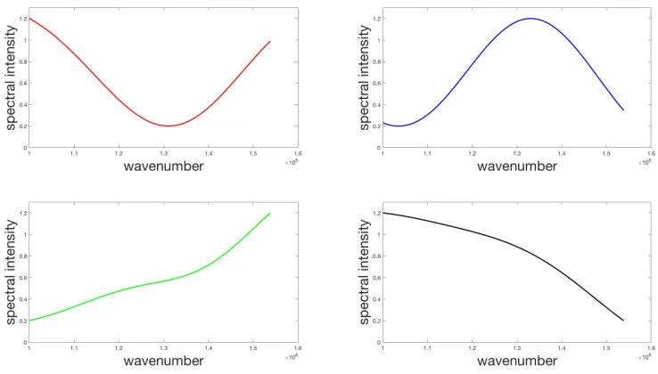
Then different smoothly varying spectra are set to each of these points. The spectrum of a

point is assumed to be one of the four functions sampled from a Gaussian ProcessGP(m, K). A Gaussian process (GP), written asX ∼GP(m, K), defines a distribution, in which the random

continuous functionX is distributed with mean functionm and covariance functionK. Since a

GP defines a probability distribution on the space of continuous functions, the spectral intensity functions can be sampled from it. Here, a very important property of GP is used: every point

in the continuous input space (domain ofX) is associated with a normally distributed random

variable; every finite collection of those random variables has a multivariate normal distribution, whose covariance matrix can be derived using the covariance functionK. Therefore, if a function

measured onN discrete points inσneeds to be sampled, aN-dimensional multivariate Gaussian

has to be defined, whose mean is the discrete realization of m. Each entry of the covariance matrix is computed by K(x, x0), where x and x0 are two of the N discrete points. Here, the

covariance function is

K(x, x0) =exp(−kdk

2

2l2 )), (2.1)

whered=x−x0,lis the characteristic length-scale parameter. Finally, the functions are sampled

from that multivariate Gaussian. After the four spectral intensity functions are generated, they

(18)

(a) 3D-spatial spiral piecewise-smooth object

(b) The 2D cross-sectional planes of the spatially smoothed spiral curve object associated with the fifth position in the other dimension

(19)

spatial location (voxel) is randomly assigned with one of the four spectral intensity functions.

Figure 2.2 shows four randomly generated spectral intensity functions withl= 3×105. Such a largel can ensure the functions’ smoothness.

Figure 2.2: Spectral intensity functions sampled from a Gaussian Process

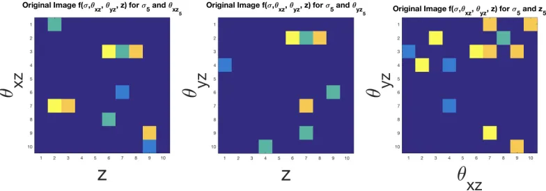
Figure 2.3 shows the ground truth of three 2D cross-sectional planes of a synthetic point

cloud with 100 sampled points in a 3D spatial datacube. The spectra of the points are

color-coded with four different colors, corresponding to the four spectral intensity functions.

Compared to the spiral curve object, this point cloud object is more difficult to be accurately

reconstructed due to the following three facts.

(a) The object is more complicated.

There are about 10 points in each 2D cross-sectional planes, but in previous spiral object,

there are only 1 or 2 points per plane. Thus what needs to reconstruct is a mazy-like pattern.

(b) The object is not spatially smooth.

No Gaussian filter is applied to the point cloud object, meaning the intensity at each location

is independent to others so that smoothness constraints can not be added between neighboring

locations.

(c) The object has more complex spectra.

(20)

Figure 2.3: Cross-sectional planes of the ground truth object with 100 random points

2.3 A specific scene

This section presents a further more complicated and specific object, which is a specific scene that consists of three bar objects. The shape of the bar is also represented using a point cloud.

As shown in Figure 2.4 (a) and (b), the three bars are placed diagonally in the spatial 3D

space. Each bar contains 32 sample points divided into 4x-y planes. The spectral intensity on each spatial location is generated using the same method as the previous point cloud object.

Figure 2.4 (c) shows three cross-sectional planes.

To adequately demonstrate the bar shape of the point cloud, the spatial resolution of the object needs to be increased. Moreover, the sampling points have been doubled: 288 sampling

points eachσ in the spectrum direction compared to the previous objects (100 sampling points

each σ). The detector size and detector resolution are also increased to improve the condition of determination. All these facts lead to a much larger linear system with a huge number of

variables to be estimated. The later chapter will show later that a simple non-parametric

repre-sentation of the object will be computationally challenging, thereby motivating the parametric reconstruction methods.

2.4 Experimental setup

To setup the experiments, there ground truth objects f(σ, θxz, θyz, z) (the object models

de-scribed above) are designed. All of these three kinds of objects are put in the same spatial

location in the modulation model with the incident angle from 45◦ to 55◦ and the distance ofz

from 1m to 4m. They have the same range of wavelength 1_σ from 650nmto 1000nm. While the object’s spatial resolution and spectrometer’s detector resolution are set to be different so as to

(21)

(a) The 3-bar object shown as a point cloud using MeshLab (this is the actual form of data the algorithm deals with)

(b) The 3-bar object shown as a mesh using MeshLab (this is a conceptual illustration of the object)

(c) The 2D cross-sectional planes of the spatially smoothed spiral curve object associated with the fifth position in the other dimension

(22)

1000×10×10×10, which means there are 1000 sampling points inσand 10 sampling points in

each spatial dimension. For the 3-bar object,the number of sampling points inσis reduced and more points are sampled in the 3D space, so that the object resolution is 100×17×17×17.

Then the corresponding measurementsg(σ, xp, yp) and the measurements matrixH(σ, xp, yp, //θxz, θyz, z)

need to be simulated. The spectrometer detector is a squared 2D plane, of which the side length varies according to the object type. The squared detector is set to be 5 cmfor the spiral curve

object, and 25 points are sampled within the detector (5 points for each spatial dimension),

and have 25 equations for each wavelengthσ. Thus the measurement resolution is 1000×5×5. The measurement matrix H is a 1000×5×5×10×10×10 6-dimensional matrix. Since the

random point cloud object is more complex, the detector size is increased to be 10×10cm2, so that g has a 1000×10×10 resolution and H matrix becomes 1000×10×10×10×10×10. For the most challenging 3-bar scene object, the measurements g becomes 100×20×20 with

a detector of 15 cm side length, so that H is 100×20×20×17×17×17.

There are various noise in imaging systems, including photon noise, dark noise, read noise, etc. It has been shown that the photon noise[3] accounts for the majority of the total noise.

Since the Poisson distribution can best model the photon noise, Poisson noise is added onto

the measurementsgbefore the reconstruction, and compare the reconstructed result to the one without noise to test the robustness of the algorithm. The mean of the Poisson distribution,

which is the square of the Signal Noise Ratio (SNR), ranges from 5 to 30 in the tests.

2.5 Conclusion

This chapter introduced three types of ground truth objects that are going to be used to

validate the reconstruction algorithm. It described the methods to generate these objects and their characteristics respectively. The spiral curves and the random point clouds will be used in

both the non-parametric and parametric data reconstruction, while the 3-bar object will only

be used in the parametric model due to its large number of variables and model complexity. It also gave the parameter settings of the SSM system for generating these ground truth objects,

including the detector size of the spectrometer, the range of incident angles and the range of

the spatial distance from the detector. Besides, it specified the spatial and spectral resolution for each kind of objects and their corresponding measurements. Additionally, it gave the range

(23)

Chapter 3

Non-parametric data reconstruction

With the given optical model and the sensor measurements, the goal is to reconstruct the object scene. This chapter introduces the technical details of the data reconstruction methods. Data

reconstruction is a widely studied topic in pattern recognition [2]. Methods like deep learning

and Bayesian inference have achieved success in many machine learning fields to solve the re-construction and inverse problems. Considering the fact that the rere-construction system is an

ill-conditioned inverse problem, it is proposed to use two optimization-based data

reconstruc-tion approaches. This chapter will introduce the first one: non-parametric data reconstrucreconstruc-tion method, with which all of the spatial/spectral variables in the objectf need to be optimized.

Then this chapter will describe an iterative numerical method used for solving such a

large-scale optimization problem. Finally, it will present the reconstructed results for the spiral curves and the random point cloud object and analyze the existing problems of the non-parametric

optimization.

3.1 Posterior optimization for an underdetermined linear

sys-tem

As mentioned in Sec. 1.1.3, the object to be recovered is the 4D data. In the discrete setting, the simplest way to represent such an object is to have one variable for each frequency component

of each spatial location; that is,f is represented by a discrete 4D data (dimension ordered by

(σ, x, y, z)) with a dimension ofM×N×N×N. In other words,fis regarded as anM×N×N×N

dimensional variable. Such a representation is called thenon-parametric representation of the

4D data.

As discussed before, the algorithm is dealing with an underdetermined linear system with more unknowns than the number of equations, so the objectf cannot be uniquely computed in

(24)

tries to estimate it from a probabilistic perspective. The algorithm uses an optimization-based

method to estimatef instead of directly solving the linear system by matrix inverse. The method is to formulate a probability distribution on the unknown objectf and perform an

Maximum-a-Posteriori (MAP) analysis [21]. The measurement matrix H can be generated based on the

SSM system, and the measurementsgcan be simulated from the synthetic ground truth object. These two given data can be the entry of the optimization method to estimate the object.

To be specific, the goal is to model the probability distributionp(f|g, H), which indicates the

probability of observing f given the measurement matrix H and the measurementsg. By the Bayes’ rule,

p(f|g, H)∝p(g, H|f)p(f). (3.1)

The posterior is proportional to the product of a likelihood term p(g, H|f) and a prior term

p(f). The goal then is to find the mode (minimizer of the negative logarithm) ofp(f|g, H). Due

to the fact that the system is an under-constraint linear system, some proper prior distributions have to be imposed on thef variable.

3.1.1 Heuristic prior assumptions

As mentioned above, the underdetermined linear system onf may lead to an infinite number of solutions. Therefore, a key step in the Bayesian analysis is to have a proper prior distribution

p(f) to regularize the recovered object. There are two heuristic assumptions to construct p(f):

the spatial smoothness assumption and the spectral smoothness assumption.

Thespatial smoothness assumption refers to the fact that in almost all situations, the

inten-sity of an object across the spatial domain tends to be smoothly varying rather than randomly

changing. This idea has been extensively applied to feature detection, image segmentation tasks [6] and image denoising [23]. In this case, it is assumed that the intensity of each frequency

component of the 4D object is varying smoothly in the spatial domain (x-y-z coordinates). In

other words, the spectral intensities of neighboring locations have strong correlation, meaning in each spatial hyperplane (the 3D space formed byx-y-z), the spectral intensity in one location

will not change too much with respect to its neighbors in any of the three spatial (x,y and z)

directions. In order to model this fact, a Gaussian distribution is imposed on the object’s three spatially directional derivatives:

p(∇xf)∝ N(0, I), p(∇yf)∝ N(0, I), p(∇zf)∝ N(0, I), (3.2)

where ∇vf is a vector containing spatial derivatives of spectral intensities for all spatial

(25)

Discrete computation of such operations will be given at the end of this section. The zero-mean

Gaussian encourages small spatial derivatives, thereby allowing spatially smoothness estimation of the object.

The spectral smoothness assumption means that for each spatial location (discretized

loca-tion of the object), its 1D spectrum should also vary smoothly across all σ planes (frequency components). Similar to the spatial smoothness situation, one possible way is to impose a

Gaussian distribution on the spectral derivatives of the object.

p(∇σf)∝ N(0, I), (3.3)

where∇_σf is a vector containing spectral derivatives for all spatial locations. Assuming the spa-tial smoothness and spectral smoothness can be modeled independently, the prior distribution

p(f) follows

p(f)∝p(∇_xf)p(∇_yf)p(∇_zf)p(∇_σf). (3.4) The negative logarithm of the prior distribution p(f), also known as the data regularization term, has the following form:

−log(p(f))∝(λ1k∇xfk2+λ1k∇yfk2+λ1k∇zfk2+λ2k∇σfk2), (3.5)

whereλ1andλ2can be viewed as the weighting factors between spatial smoothness and spectral

smoothness, and they are essentially related to the Gaussian distributions’ standard deviations.

Normally the two weighting factors should be different, because the spatial smoothness and spectral smoothness are not commensurable. The spatial smoothness priors may be disabled

by settingλ1 to zero for the random point cloud and 3-bar scene objects, because point clouds

inherently do not satisfy the spatial smoothness assumption. The spectral smoothness constraint is always in use for all objects, but λ2 may be set to different values for different spectral

smoothness levels and different spectral resolutions. For example, a larger λ2 is needed to

model a higher smoothness level of the spectral intensity function with a largerl in Eq. 2.1.

3.1.2 Likelihood

GivengandH, the estimatedf should satisfy the linear relationship in Eq. 1.1. This corresponds

(26)

in a convolution format, the negative logarithm of the likelihood distribution can be defined as

p(g, H |f) ∝ exp(− X

σ,xp,yp

kg(σ, xp, yp)−H(σ, xp, yp)⊗f(σ)k2) (3.6)

−log(p(g, H |f)) = X

σ,xp,yp

kg(σ, xp, yp)−H(σ, xp, yp)⊗f(σ)k2+ constant. (3.7)

Note that this term is often referred to as the data matching term, because it encourages the

estimated f to better explain the observed data g and H. The following text slightly abuses this notation by denoting the linear relationship simply as g−Hf.

g(σ, xp, yp)−H(σ, xp, yp)⊗f(σ)→g−Hf (3.8)

3.1.3 MAP analysis

Maximizing the posterior of Eq. 3.1 is equivalent to minimize its negative logarithm, which

corresponds to the following objective function:

arg min

f −log(p(f|g, H)) (3.9)

−log(p(f|g, H)) =kg−Hfk2+ (λ1k∇xk2+λ1k∇yk2+λ1k∇zfk2+λ2k∇σfk2). (3.10)

Here only the L2 norm is used in the data matching and regularization term. This naturally

corresponds to the form of the Gaussian logarithm. The Gaussian distribution is preferred in many other applications due to its many elegant properties. One particular reason is that the

quadratic term of L2 norm is easy to optimize numerically. However, it is known that for some

specific situation, L1 norm is more desirable due to the fact that it can induce sparse solutions, which might be a more appropriate assumption for some applications. The downside of using

the L1 norm is that numerical methods for L1 optimization are generally not well developed.

This application chooses to use the L2 norm instead of the L1 norm.

Discrete computation of directional derivatives.

In the discrete situation, the derivatives are approximated by computing finite difference in

the four directions as illustrated in the following. Using the non-parametric presentation of the object,∇_vf is computed by

(27)

wherev can be either one of {σ, x, y, z}

∇σf(i, j, k, p) =f(i+ 1, j, k, p)−f(i, j, k, p) (3.12)

∇xf(i, j, k, p) =f(i, j+ 1, k, p)−f(i, j, k, p) (3.13)

∇yf(i, j, k, p) =f(i, j, k+ 1, p)−f(i, j, k, p) (3.14)

∇_zf(i, j, k, p) =f(i, j, k, p+ 1)−f(i, j, k, p). (3.15)

3.2 The L-BFGS numerical method

After having an objective function for the data reconstruction model, the next step is to find an

appropriate numerical optimization method. It can be seen that the above objective function

Eq. 3.9 is quadratic. If the data dimension is small, the optimality condition can be directly written down as another linear system with the linear matrix operator being the Hessian matrix.

However, if the data dimension is large, methods that require computing or inversing the Hessian of the objective function will be too time-consuming. Since the ultimate goal is to recover a 4D

point cloud dataset with more than 10GB variables, it will be too expensive to directly compute

the Hessian.

There are some popular quasi-Newton methods such as symmetric rank-one (SR1),

Davidon-Fletcher-Powell (DFP) and Broyden-Fletcher-Goldfarb-Shanno (BFGS) algorithm, which can

approximate Hessian with faster progress [26]. An advanced BFGS algorithm, Limited-memory BFGS (L-BFGS) [19] is applied, which is especially proposed for optimizing large scale problems

with only a limited computer memory. Instead of computing and storing a densen×n

approxi-mation to the inverse Hessian (nbeing the number of variables in the problem), L-BFGS stores only a few vectors that represent the Hessian approximation implicitly. Thus, it can achieve

fast and accurate computational results for this problem. It used to cost 1.5 hours to run a

preliminary 3D object with the data scale of only 80 MB. Using L-BFGS, it can reduce the running time of 80 MB data to 5 minutes, which is a huge improvement.

3.3 Reconstruction results

This section presents two experimental results using the non-parametric posterior optimization

method. The first experiment is to verify the necessity of both spatial and spectral smoothness

assumptions using the spiral curves object with a lower spectral resolution (100 spectral sam-pling points per location). The second one is to analyze the reconstruction results of the spiral

curves and random point clouds with a higher resolution (1000 spectral sampling points per

(28)

Validation tests of the spatial and spectral smoothness assumptions

In order to validate the two prior assumptions, the algorithm first recovers the spiral curves without using any regularization terms, meaning that it simply perform a matrix inverse

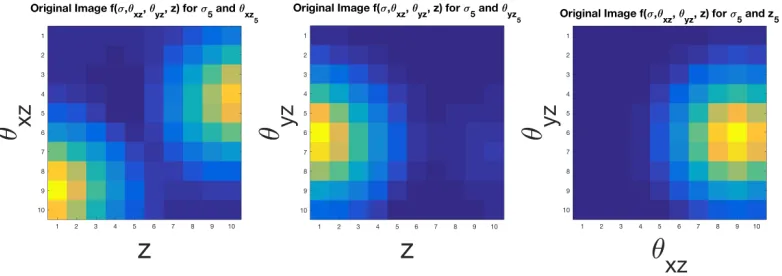
(pseudo-inverse) to the underdetermined linear system. Figure 3.1 shows six cross-sectional

planes (three spatial cross-sectional planes in Figure 3.1(a) and three spectral cross-sectional planes in Figure 3.1 (b)) of the ground truth synthetic object for reference. Note that,

Fig-ure 3.1 shows the ground truth for all the rest reconstruction results of the spiral curves object.

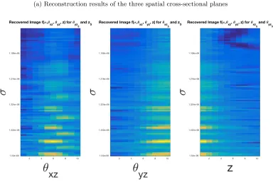
Figure 3.2 shows the reconstruction results by pseudo-inverse for the same six cross-sectional planes as in Figure 3.1. It can be seen that without any spatial and spectral regularization, a

direct matrix inverse does not yield meaningful results. Neither spatial nor spectral planes can

be recovered to assemble the ground truth.

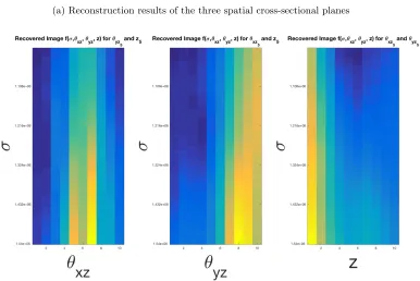
Then Figure 3.3 shows the reconstruction results assuming spatial smoothness only. It can

be seen that the three spatial cross-sectional planes are recovered much better. However, the

spectra are still problematic due to the lack of constraints.

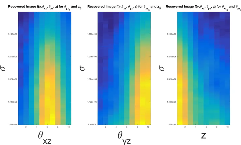
However, when assuming spectral smoothness only, it can achieve more accurate results in

both the spatial and spectral cross-sectional planes as shown in Figure 3.4. That means the

spectral prior alone is more effective than the spatial prior alone.

If using both spatial and spectral assumptions, the all six cross-sectional planes can be

very well recovered as shown in Figure 3.5, which proves the importance of the two prior assumptions used in this method. The accuracy of the algorithm is quantified with two kinds

of Mean Square Errors (MSE). One MSE is the overall MSE, which is computed by averaging

the squared intensity error over all spatial locations and frequency components. The other one is sparse point MSE, which is computed only on those locations with object sampling points.

Besides MSEs, the running time is another important aspect needs to be investigated. The goal

of this algorithm is to achieve high accuracy with limited computational time. The overall MSE of the final experiment (with both prior assumptions) is shown in Figure 3.5 is 0.85% (0.85%

of the maximum intensity in the normalized object). The sparse point MSE is 10.08%. Since

the 4D object is extremely high-dimensional, the running time of the optimization was about 1.5 minutes on an i7-3770k 3.50GHz Intel CPU processor.

Reconstruction results of high resolution objects

When using the high resolution 1000×10×10×10 object, the system have much more unknown variables in spectral dimension. As shown in Figure 3.6, the non-parametric method

cannot reconstruct well even with both prior assumptions. The overall MSE (0.92%) and the

parse point MSE (10.17%) are both larger than the low resolution results and the running time is also much longer: 6 minutes.

When it goes to the random point cloud, the object is no longer spatially smooth. Therefore,

(29)

(a) Three spatial cross-sectional planes of the ground truth spiral curves object

(b) Three spectral cross-sectional planes of the ground truth spiral curves object

(30)

(a) Reconstruction results of the three spatial cross-sectional planes

(b) Reconstruction results for the three spectral cross-sectional planes

(31)

(32)

(33)

(34)

(35)

matching and spectral smoothness terms. Figure 3.7 shows the ground truth for the random

point cloud object and Figure 3.8 gives the reconstruction results.

The overall MSE of this experiment is 1.73%, and it also takes nearly 15 minutes on the

optimization.

3.4 Conclusion

This chapter described a posterior optimization model and gave the derivation of the objective

function for the non-parametric presentation of the 4D data. It also presented the reconstruction results using this non-parametric optimization approach and showed the importance of the

two prior assumptions being incorporated. The MSEs indicated that the algorithm can work

well on both spatially smooth and non-smooth objects with relative lower resolution in the spectrum. However, the remaining problem is that the optimization with the non-parametric

data representation cannot perform well on the objects with a higher resolution and it is too

inefficient. Usually 100 iterations in L-BFGS require more than 15 minutes to reconstruct an object with the scale of 380M B(this is only ₄₀1 of the largest possible scale in this thesis). With this in mind, a more computationally efficient method will be introduced in the next chapter

(36)

(a) Three spatial cross-sectional planes of the ground truth random point cloud object

(b) Three spectral cross-sectional planes of the ground truth random point cloud object

(37)

(38)

Chapter 4

Parametric data reconstruction

It has been noticed that a non-parametric representation (one variable per frequency and per location) offwill contain a large number of variables. This leads to a high-dimensional

optimiza-tion problem that is computaoptimiza-tionally intensive even with the Hessian approximaoptimiza-tion method.

To handle this situation, this chapter further explores the spectral smoothness idea mentioned in Sec. 3.1.1 with the reparameterization trick. Given a function f represented in a canonical

domain, the reparameterization off refers to the procedure of transforming its representation in

some other domains, such as the Fourier domain, the Wavelet domain [5] and the Reproducing-Kernel-Hilbert-Space (RKHS) [1]. The intention of such reparameterization tricks is that the

function can be compactly represented in the new domain with much fewer coefficients; that is,

after projectingf into the new coordinate system (not necessarily orthonormal), the projection coefficients are mostly zero or near-zeros. Therefore, the data components associated with the

near-zero coefficients can be directly discarded, and the reconstructed function with the limited

number of coefficients can still highly approximate the originalf.

Therefore, given a 4D f, the idea is to reparameterize the spectrum of each spatial location

to reduce the number of variables in the spectral direction. As mentioned before, in most

cases, the spectra are smoothly varying and they can be compactly represented in many other domains. The reparameterize spectra are particularly chosen instead of reparameterizing spatial

components because in some cases, e.g., the point cloud, the spatial components are not smooth.

This chapter will investigate two reparameterization methods: RKHS and B-spline. Again, the method will still incorporate the previous prior assumptions, the posterior optimization

framework and the L-BFGS numerical method. Such methods are called asparametric methods

because they work with the data form after reparameterization. Besides the spiral curves and the random point cloud object, this chapter will use the parametric method to reconstruct the

(39)

both non-parametric and parametric methods with different objects of different scales.

4.1 The RKHS reparameterization model

To reduce the number of variables, the first model applied to reparameterize the function is

the RKHS space spanned by the eigenfunctions of a Gaussian kernel. The idea is that the

eigenfunctions sorted by the eigenvalues show the nature of multi-scale smoothness, where the first eigenfunction is a very smooth function and the last eigenfunction is a fast oscillating

function. This leads to a fact that when projecting a smooth function into the RKHS space, the projection coefficients decay very fast. In other words, it can just approximate a smooth

function using the very few coefficients associated with the first few eigenfunctions [1]. The

Gaussian kernelK is given in Eq. 2.1. By Mercer’s theorem,K may be written in terms of the eigenvalues and continuous eigenfunctions as

K(x, x0) =

∞

X

i=1

λiφi(x)φi(x0)T, (4.1)

where λi and φi(x) are eigenvalue and eigenfunction pairs. The RKHS is spanned by linear

combinations of these eigenfunctions[12].

Therefore, for each spatial location, the spectral function f(·, x, y, z) can be then approxi-mated as:

f(·, x, y, z)≈Φα(x, y, z), (4.2)

where the vectorα(x, y, z) = [α0, ..., αN] is the coefficients vector for the firstN eigenfunctions,

and Φ represents a matrix of the firstN eigenfunctions. With this reparameterization,α is the

new representation of a spectrum in the RKHS space. Typically N is much smaller than the dimension inσ, thereby enabling reduction in the number of variables. For example, 4.1 shows

the result of projecting a simple linear function onto the first 1000 eigenfunctions. It can be

seen that the projection coefficients are decaying very fast, which means the first few coefficients with their eigenvectors can precisely approximate the original function.

Therefore, if reparameterizing the spectrum of each location only using the first 50

eigen-functions, only a 50-tuple vector for each object location needs to be recovered, whereas in the previous non-parametric representation the spectrum is a 1000-tuple vector. Now the

ob-jective function in Eq. 3.10 is changed to optimize the α vectors for every spatial location.

With a little abuse of notation, now α is used to represent the reparameterization vectors for all spatial locations and use α(x, y, z) to represent the N-tuple alpha vector for a particular

(40)

(41)

reparameterization, the likelihood term becomes

kg−HΦαk2. (4.3)

The spectral smoothness assumption is inherently given by the RKHS reparameterization: it

turns out that the way for measuring a function’s smoothness in the RKHS space is to use the

so-called k-norm. Assume β is an RKHS reparameterization coefficient vector, its k-norm is defined as

kβk_k=

N

X

i=1

β_i2 λi

, (4.4)

where the set of{λi} is the corresponding firstN eigenvalues. The spatial smoothness, on the

other hand, is then measured by the k-norm of the difference between the two α vectors of

neighboring spatial locations. It is defined that

k∇α(x, y, z)kk=k∇xα(x, y, z)kk+k∇yα(x, y, z)kk+k∇zα(x, y, z)kk, (4.5)

where∇_xα(x, y, z) is the subtraction of the twoα vectors between neighboring locations in the

x direction, i.e.

∇xα(x, y, z) =α(x+ 1, y, z)−α(x, y, z), (4.6)

and the same rule applies for ∇_yα(x, y, z) and ∇_zα(x, y, z). Therefore, the overall objective function becomes

arg min

α kg−HΦαk

2₊_λ 1

X

x,y,z

k∇α(x, y, z)k_k+λ2

X

x,y,z

kα(x, y, z)k_k, (4.7)

The same L-BFGS method can be applied here to optimize the α variables. However, the

dimension ofα is much smaller than that of the non-parametric form.

4.2 The B-spline reparameterization model

The second model used is to reparameterize the spectrum of the object using B-spline coeffi-cients. The smooth nature of the spectrum allows us to adopt a low-order polynomial

approx-imation with a limited number of control points (knots). Similar to the previous RKHS idea,

instead of optimizing over a high-dimensional non-parametric domain associated withf, it only needs to optimize over a lower-dimensional B-spline coefficient space.

A B-spline of order nis a piecewise polynomial function of degree< n[9]. The places where

(42)

B-splines of that degree. Assume the B(x) is a spline with degreen and there are K interior

knots, the following equation shows the B-spline reparameterization:

B(x) =

K+n

X

i=0

αiBi,n(x), x∈[t0, tN+1], (4.8)

where n is the degree of B-spline, K is the number of interior knots, and αi are the control

point coefficients. The ith B-spline basis function can be defined recursively using the Cox-de Boor recursion formula:

Bi,0(x) =







1 ifti≤x < ti+1

0 otherwise.

(4.9)

Bi,k(x) =

x−ti

ti+k−ti

Bi,k−1(x) +

ti+k+1−x

ti+k+1−ti+1

Bi,k−1(x). (4.10)

Usually, more knots should be put in regions where the functions are changing more rapidly. Since in this problem the spectrum is smoothly varying, the knots can be equidistantly placed.

For any given set of knots, the B-spline is unique, Figure 4.2 shows a series of B-spline functions

with 10 knots and an order of 4. Each different color of the polynomial in the figure represents a different basis spline.

(43)

Therefore, for each spatial location, the 1D spectrum function of f at any given local can

be then approximated as a linear combination of B-splines. Similar to the previous RKHS formulation, B is used to denote a matrix storing the N B-splines and useα(x, y, z) to denote

the B-spline coefficients of a particular spatial location (just like in the previous sectionα(x, y, z)

is used to denote RKHS coefficients). Then Eq. 4.8 can be rewritten as

f(·, x, y, z)≈Bα(x, y, z), (4.11)

Again, the following text will use α to denote the set of B-spline coefficients for all spatial

locations. Since the method is using a limited number of knots for generating the B-splines, the dimension of α is much smaller than the non-parametric representation, and the number

of unknown variables to be estimated is highly reduced.

Now the objective function in Eq. 3.10 has to be rewritten in terms of B-spline coefficients

α. This part follows exactly to the previous section except that the RKHS coefficients are

re-placed by B-spline coefficients. For the likelihood term, it is obvious that Eq. 4.11 and Eq. 3.8 yield a composite linear relationship, which is denoted by HBα. For the spatial smoothness

term, the directional derivatives of B-spline coefficients should be penalized instead of spectral

intensities. Lastly, the B-spline reparameterization already implicitly guarantees the spectral smoothness by constraining the 1D spectrum to be a low-order polynomial. However, an

ad-ditional regularization kα(x, y, z)k2 _{is put to penalize too large B-spline coefficients to avoid}

overfitting. The objective function becomes

arg min

α kg−HBαk

2₊_λ 1

X

x,y,z

k∇α(x, y, z)k2₊_λ 2

X

x,y,z

kα(x, y, z)k2_. _(4.12)

4.3 Reconstruction results

This section will provide the reconstruction results for three different experiments with their

goals being (a) to compare the RKHS and B-spline models (b) to test the robustness of the al-gorithm under Poisson noise and (c) to perform a thorough comparison between non-parametric

and parametric methods.

Comparison tests of the RKHS and B-spline reparameterization models

Since the emphasis of this chapter is the reparameterization trick, the first validation test

is to compare the performance of two parametric methods: RKHS and B-spline. Here the

experiment uses the spiral curves object and assumes both spatial and spectral smoothness. The following Figure 4.3 shows the reconstruction results using the RKHS reparameterization

model with 10 eigenfunctions, with the overall MSE 1.33%, the sparse points MSE 10.45%,

(44)

can be seen that the spatial cross-sectional planes can be almost recovered, but RKHS can not

accurately represent the spectral smoothness. Therefore, RKHS is not an appropriate orthogonal basis for the reparameterization purpose.

Figure 4.3: Reconstruction results for spiral curves object using the RHKS parametric method

While, as shown in Figure 4.4, B-spline performs well in both spatial and spectral

(45)

7.97%), and the running time is 2 minutes for 100 L-BFGS iterations, which are all better than

the results form RKHS model. Thus the thesis will use the B-spline reparameterizaton model for the following experiments.

Then the B-spline reparameterization method is used to recover the random point cloud

object. Figure 4.5 shows the reconstruction results, while the ground truth can be found in Figure 3.7. The overall MSE for the result without noise is 0.14% (sparse point MSE 3.62 %)

and the time cost is 7 minutes.

Due to the reduction in the number of unknown variables, the large data scale of the 3-bar scene object can be handled using the reparameterization trick. Figure 4.6 gives the ground truth

of the six cross-sectional planes of the 3-bar object and Figure 4.7 shows the six corresponding

reconstruction results. The overall MSE is 0.12% (sparse point MSE 10.82 %), and running time are 40 minutes for 100 iterations.

To visualize the sparse point MSE more intuitively, the ground truth and recovered spectral

intensity on one spatial location from the results in Figure 4.6 and Figure 4.7 are plotted in Figure 4.8. The two spectral intensity functions are very close to each other, where the blue

line denotes the ground truth spectrum and the green line is the recovered one.

Robustness tests with Poisson noise

The second experiment is to validate the robustness of the B-spline-based parametric data

reconstruction algorithm. As described in Sec. 2.4, the measurements are polluted with Poisson noise before the optimization. Taking the example of the 3-bar object, the algorithm use the

ground truth object to simulate the measurements and add Poisson noise with SNR = 30. It

uses the B-spline-based parametric method to recover the 3-bar object in Figure 4.6. Figure 4.9 shows the reconstruction results with Poisson noise (SNR = 30). The MSE for the result with

noise is 0.26%. It can be seen that visually the recovered object still looks reasonable and the

MSE value is only increased slightly, so it can be claimed that this algorithm gives equally reasonable results in dealing with the Poisson noise at this SNR level. The running time is also

similar.

To give an overall view of the robustness tests, Figure 4.10 summarizes the MSE of different SNR settings (ranging from 5 to 30) for all three objects using the B-spline-based

paramet-ric optimization. It can be seen that the performance of the method drops with lower SNR.

However, but the algorithm can still achieve reasonably good MSE at the level of SNR = 30.

Comparison tests of non-parametric and parametric methods

Finally, this section will illustrate the advantages of the B-spline-based data reconstruction

method by comparing the accuracy and efficiency with the non-parametric method. The above reconstruction figures can give us a qualitative comparison, while the following figures and

tables will provide a quantitative results.

(46)

(47)

(48)

(a) Three spatial cross-sectional planes of the ground truth 3-bar object

(b) Three spectral cross-sectional planes of the ground truth 3-bar object

(49)

(50)

Figure 4.8: The spectral intensity of 3-bar ground truth and reconstructed results using the B-spline parametric method

most critical advantage is its higher computational efficiency. The parametric method can be much more time-consuming at any data scale level as shown in Figure 4.11. The vertical axis

means the running time with the unit os seconds and the horizontal axis represents different

data scales. The gap between the running time becomes even larger when the data scales up. Although the parametric method costs less running time and saves memory, it can provide

even better reconstruction results as the non-parametric method. Figure 4.12 shows the overall

MSEs for different data scales using these two methods.

4.4 Conclusion

Considering both of the limited computer memory and high-dimension object datasets, the

algorithm proposed two reparameterization methods to reduce the number of variables in the posterior optimization. One is the RKHS model, which uses the first few eigenfunctions of a

Gaussian kernel to approximate a smooth function. The other one is the B-spline model, which reparameterizes a function by some low-order polynomials. According to the experiment results,

the B-spline model is better at modeling the continuous spectra. Then it demonstrated the

re-construction results of three kinds of objects using this B-spline-based method with and with-out the Poisson noise. In the end, it compared the parametric method with the non-parametric

method from the aspects of accuracy and efficiency to prove the advantage of using

(51)

(52)

(53)

(54)

(55)

Chapter 5

Conclusion and discussion

This thesis investigated a reconstruction algorithm for 4D object-space data using the SSM technique and validated the algorithm using synthetic ground truth objects. The SSM technique

is a hyperspectral imaging technique applied for far-field target detection in passive remote

sensing systems.

The first problem encountered is that the SSM system is an underdetermined linear

sys-tem. The system has much fewer number of equations from the optical and modulation model

than the number of unknown variables in the scene object, so it cannot uniquely compute the unknown variables in a closed form. Therefore, the algorithm models the problem from a

probabilistic point of view. The algorithm has proposed two proper prior distributions on the

object scene and formulated a posterior optimization to solve the inverse problem. The second challenge is the optimization efficiency. When trying to reconstruct the 4D scene with much

larger data scale (more than 10 GB), one problem is the computer memory is not large enough

to handle the optimization, and the computational time is also too slow; the other problem is that with limited detector size this system becomes further ill-posed for such a large scale

ob-ject scene. Thus the data is reparameterized by proob-jecting it into some other domain and using

only a few projection coefficients. In particular, much fewer variables are used to represent the continuous spectra of the object. Such a reparameterization trick can reduce the optimization

memory consumption by 95%. Through the experiments on several different

reparameteriza-tion models, it proves that the B-spline reparameterizareparameteriza-tion can best reconstruct the object with efficient computation.

The novelty of the algorithm are: (a) it proposes to incorporate proper prior assumptions to

the object scene so that it can solve effectively the underdetermined linear system by an inverse optimization (b) it proposes to use RKHS basis functions and B-spline polynomials to represent