Article
A Distributed Optimization Method for Energy
Saving of Parallel-Connected Pumps in HVAC
Systems
Xuetao Wang1, Qianchuan Zhao1* and Yifan Wang1
1 Department of Automation, BNRist, Center for Intelligent and Networked Systems, Tsinghua University, Beijing 100084, China
* Correspondence: [email protected];
Abstract: The energy saving problem of parallel-connected pumps in heating, ventilation, and air-conditioning (HVAC) systems has received an increasing attention in recent years. While many pump optimization methods are proposed and show great performance, pumps are not always energy saving and lack flexibility. In this paper, we propose a distributed control algorithm for parallel-connected pumps in HVAC systems. Based on a spanning tree of the intelligent nodes and a population of potential solutions, the algorithm makes the optimal control decision for pumps to minimize the energy consumption and meet the system demand. The theoretical analysis on convergence of the algorithm is established. Unlike traditional control structure, the whole system is fully distributed and each pump is controlled by an intelligent node that runs the identical control code and coordinates with other nodes through direct data exchange. Simulation experiments on 6 parallel-connected pumps are provided for different working cases to demonstrate the effectiveness of the proposed algorithm and compare with other four methods. The results show that our algorithm strictly satisfies the demand constraint and presents good energy saving potential, the convergence guarantee, the flexibility. The maximum energy saving can be up to 29.92%. Besides, the hardware test clearly presents that our algorithm can perform on low-cost Raspberry Pi3 and reduce the system cost.
Keywords:Distributed; Parallel-connected pumps; Speed Ratio; Optimal control; Spanning tree
1. Introduction
The heating, ventilating, and air-conditioning(HVAC) system makes up approximately 50% of building energy consumption and 20% of total energy consumption [1]. Parallel-connected pumps, which provide as wide flow range as possible, are the main power consumer devices in HVAC systems. The report of European Commission shows that pump systems account for nearly 22% of the energy consumed by electric motors in the world [2]. The energy consumption of pumps to transport energy into rooms is responsible for a significant portion of HVAC energy consumption [3]. It accounts for about 40% of the total HVAC energy use [4]. These numbers demonstrate that the system with parallel-connected pumps has great potential for energy saving and there is an increased attention associated with the operation of pumps. Many advanced computer control systems have been implemented in HVAC systems [5]. How to optimally control the number of running pumps and corresponding speeds is important to reduce the total energy consumption and exactly meet the demand.
Researchers have proposed various pump optimization strategies to reduce the energy consumption [8]-[23]. These methods play important roles and help human operators to save much
仇ಞ
仇ಞ
仇ಞ
仇ಞ
ᵰ㓺
ᵰ㓺
ᵰ㓺
ᵰ㓺
Ჰ㜳㢸⛯ࡓခौ ީؗᚥ
䳅ᵰ⭕ᡆṭᵢ⛯θ䘑 㺂ީ䇗㇍
㔉ᶕϋ
ੇ䛱ቻՖ䙈ᖉࢃṭᵢ ⛯Ⲻީؗᚥ
ṯᦤ䛱ቻਃ侾䘑㺂с ж↛䇗㇍
䛱ቻ
⭕ᡆ᯦Ⲻ ṭᵢ⛯ Ჰ㜳㢸⛯仇
ಞ䗉࠰ᓊ仇⦽
߭পຊ AHU
Group of pumps
Group of chillers Group of controllers
Valve
Water Collector
Water Segregator
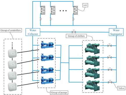
Figure 1.The distributed control framework for parallel-connected pumps.
energy in systems with parallel-connected pumps[10][13]. However, there is still room to improve existing methods. For example, sometimes, people observe frequent adjustments of the terminal air-handling units in HVAC system caused by the mismatch of flow rate demand [12]. Furthermore, without guarantee of optimality, pumps under control of existing algorithms still have energy saving potential. In addition, some of the pumps may be in maintenance (the interval of maintenance could be as long as 3 months [27]) or break down occasionally. As a result, how to adapt to such situations and continue to work in a energy saving way for pump systems might become a major challenge.
In this paper, we consider a distributed pump system as presented in Figure1and extend our previous work [6]. Our previous work only considers controllers connected in the chain topology which cannot be applied to other topologies. Here, motivated by the distributed and peer-to-peer algorithm framework proposed in [7], we put forward a novel distributed optimization method that is suitable for general topologies and establishes theoretical convergence results. Our method consists of two parts: First, in order to process the network information, we apply the breadth first search algorithm to construct a tree to exchange message. Second, all nodes coordinate with each other and randomly sample a population of speed ratios. In addition, we prove that our method has the guarantee of convergence. Based on a numerical example of pump systems, we compare our approach with other methods. It turns out that our method is able to exactly satisfy the actual demand, minimize energy consumption and has good flexibility. The hardware testing shows that our method can perform on low-cost Raspberry Pi3 and reduce the cost when applied in practical systems.
algorithm. To demonstrate the advantages of the new algorithm, in Section6, we show numerical results of the algorithm and compare it with the state of art algorithms. We also study the flexibility of the algorithm and test the algorithm on hardware platform. In Section7, we conclude the paper.
2. Literature review
There are plenty of studies on pump energy saving control and optimization. By investigating the existing papers, we summarize them into four groups including rule based methods, mathematical programming, heuristic methods and distributed methods as shown in Table1. The first three groups are based on the centralized control framework which replace the group of controllers as shown in Figure1with a single controller. The last group is based on the distributed control framework as presented in Figure1.
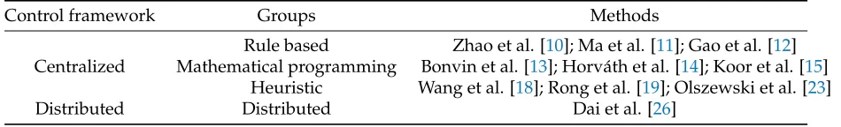
Table 1.Optimization methods for the system with parallel-connected pumps.
Control framework Groups Methods
Centralized
Rule based Zhao et al. [10]; Ma et al. [11]; Gao et al. [12] Mathematical programming Bonvin et al. [13]; Horváth et al. [14]; Koor et al. [15]
Heuristic Wang et al. [18]; Rong et al. [19]; Olszewski et al. [23]
Distributed Distributed Dai et al. [26]
2.1. Rule based methods
In the pump system, the operation still depends on human operators to manage pumps. To tackle this problem, some methods have been conducted on adjusting pump working, including on-line adaptive control [8] and group control strategy [9]. Zhao et al. [10] defined the most unfavorable thermodynamic loop and used the variable differential pressure set point control strategy of pumps. The test results saved 47-58% water pump power consumption. Ma et al. [11] developed the pressure drop models for water networks and formulated an optimal pump sequence control strategy. The number of pumps in operation was set according to their power consumption and maintenance costs. In addition, Gao et al. [12] proposed a fault-tolerant and energy efficient sequence control strategy (SC) for chilled water pump systems with a differential pressure set-point. The strategy ensured that the water flow of secondary loop met the primary loop. There was a series of operational problems for the terminal air-handling units and chillers due to the ungratified flow rate demand. Rule based methods are simple and show great performance to meet the demand. The accurate model of pumps is not needed in [10] [12]. These methods are widely used in practical engineering. Sometimes pumps cannot work in the most energy efficient way because of the non-optimal working point.
2.2. Mathematical programming methods
characteristics. Two small benchmark networks showed that the method was suitable for pump operations with lower energy costs. To develop an energy-oriented optimal control solution, Jepsen et al. [17] recommended a method to minimize the energy consumption of pump stations by two steps: First, the energy consumption for a pre-selected set of active pumps were formulated as a convex optimization problem, then the problem of choosing the number of active pumps was solved by a convex solver. The proposed solution presumed the performance curves remaining constant over time. Inspired by [17], we adopt the sequential least squares programming algorithm (SLSQP) to compare with our method. The sequential least squares programming algorithm has better computing efficiency [25]. These mentioned mathematical programming algorithms increase the ability to obtain the near-optimal solutions. Due to the equality constraints, there are some deviations to meet the demand. These methods are suitable only for specific systems and lack flexibility.
2.3. Heuristic methods
Considering the complexity of the problem, some researchers have turned their attention to heuristic optimization methods. By adopting the genetic algorithm, Wang et al. [18] proposed a bi-objective pump scheduling approach. Rong et al. [19] presented a crowding genetic algorithm to decide optimal pump configuration. Cimorelli et al. [20] studied the optimal regulation of pump systems by the genetic algorithm. In addition, Barán et al. [21] introduced a multi-objective evolutionary algorithm to solve the optimal pump scheduling problem with four objectives. Hashemi et al. [22] introduced an ant-colony optimization method to improve the optimization process and reduced the feasible solutions in the search space. The optimization process was repeated many times leading to different costs and the lowest cost was selected. In order to enhance energy conservation and analyze control strategies, Olszewski et al. [23] studied three different strategies for complex pumping stations with genetic algorithm (GA) and pointed that minimizing power consumption was the most energy efficient. The ungratified flow rate was affected by the population size. The heuristic optimization methods are powerful tools to solve the optimization problem without any derivatives and continuities assumption. The above methods adopt the advantage of population sampling to solve these combination problems. However, these methods lack convergence guarantee and cannot be used to assess the minimum energy. Under equality constraints, these methods are hard to find a feasible solution. If the system with parallel-connected pumps changes, they need to do the algorithm again.
2.4. Distributed methods
Recently, we proposed a new building control architecture Insect Intelligent Building (I2B)[7]. This new distributed control framework is convenient for pump units. It is open, flexible and has a low configuration cost. There are some early attempts to carry out the distributed control in HVAC systems. Liu et al. [24] developed a decentralized optimization algorithm for optimal set point control for HVAC systems. Dai et al. [26] introduced a novel decentralized transfer algorithm (TA) as a solution to a typical control problem for parallel-connected pumps in HVAC systems. In fact, the idea of distributed control or optimization has been applied widely in other large engineering systems such as the distributed multi-area economic dispatch for active distribution networks [28], or multi-agent traffic light control systems [29].
be optimal and extra energy is consumed. To our best knowledge, the algorithm introduced in this paper is the first effort to address above challenges at the same time.
3. Problem formulation
Consider the control of parallel-connected pumps in an HAVC system as shown in Figure1. We assume that there aremcentrifugal variable-speed pumps connected in parallel and the size of pumps may be different. The demand is a stable value during a period of time (for example one hour as given in paper [11]). Our problem is to optimize the number of running pumps and their speed set-points to meet the demand with minimum energy consumption. We also assume that underlying controllers such as those given in [2] can regulate pump speed to the new set-points in real time.
3.1. Pump models
Let us first formulate the relationship between pump speed and pump energy consumption. There are various methods to establish pump model in application, such as dynamic pump model [30], pump approximation model [23]. In order to obtain better precision and convenient calculation, we choose polynomial functions to reflect pump characteristics. It is vital to know pump characteristics to implement optimal pump control. To describe a pump, we need to consider relationships between pump head, flow rate, and efficiency. When pumps work at their rated speeds, the relationships can be indicated by the equations as below.
Hi =aP1,iQ2i +aP2,iQi+aP3,i (1) ηi =bP1,iQ2i +bP2,iQi+bP3,i (2)
Pi=
ρgQiHi
1000ηiηM,iηVFD,i
(3)
We useHito denote the head of pumpi,i =1, 2, . . . ,mwheremis the total number of pumps.
Qiis the flow rate of pumpi.ηiis the mechanical efficiency,Pi is the power consumption of pump
i. Pi depends on three sub-efficiency variables, including the mechanical efficiencyηi, the motor
efficiencyηM,i, the variable frequency efficiencyηVFD,i. TheaP1,i,aP2,i,aP3,i,bP1,i,bP2,i,bP3,iare pump
performance parameters. These parameters in the equations may be accessed by the pump performance curves or actual measurement data. The data is measured when pumps work at the rated speed. If we obtain the data, it is possible to utilize the least square method to fit the polynomial functions.
We usenito denote the actual speed of pumpi.n0,iis the rated speed of pumpi. We define speed
ratioωito depict the ratio between the actual speed and the rated speed.
ωi = ni
n0,i
(4)
In general, the pump performance parameters are related to the speed and the operating conditions. When pump works in variable speed status and the operating conditions do not change, we can attain a series of pump characteristic curves through the pump affinity laws [31], as presented in Equation (5).
Qi(n0,i) =
Qi(ni) ωi
Hi(n0,i) =
Hi(ni) ω2i
ηi(n0,i) =ηi(ni)
WhereQi(n0,i)is the rated flow rate at rated speedn0,Qi(ni)is the actual flow rate at actual speed
ni.Hi(n0,i)is the rated head at rated speedn0.Hi(ni)is the actual head at actual speedni.ηi(n0,i)is
the rated mechanical efficiency at rated speedn0. Using the pump affinity laws and Equations (1)(2), we can reach the equations of pump head and flow rate, efficiency and flow rate at a speedniincluding
rated and non-rated, which are as below.
Hi =aP1,iQi2+aP2,iωiQi+aP3,iωi2 (6)
ηi=bP1,i(
Qi ωi )
2
+bP2,i(
Qi ωi
) +bP3,i (7)
Although paper [32] indicated thatηM,i,ηVFD,i depended onωi, when the speed ratios meet
0.4≤ωi ≤1,ηM,i,ηVFD,icould suppose to be constants. The reason is thatωihas little influence on
them. Therefore, we can dispense with the impact ofηM,i,ηVFD,iand only consider the mechanical
efficiencyηi. As a result, the pump power consumption equation can be rewritten as below.
Pi=
ρgQiHi
1000ηi
(8)
3.2. Optimization problem formulation
Now let us formulate the pump speed ratio optimization problem (PSROP).[Problem 1. Pump Speed Ratio Optimization Problem (PSROP)]
min ωi,i∈{1,2,...m}
m
∑
i=1Pi(ωi) (9)
s.t. H0= Hi (10)
Q0=
m
∑
i=1Qi (11)
ω− ≤ωi≤1orωi =0, i∈ {1, 2, ...,m} (12)
The objective function presents that the optimization objective of this paper is to minimize the total power consumption of pumps in parallel. The objective function indicates that we should try to find a combination ofωito content the corresponding constraints at the lowest energy consumption.
Constraint (10) is the equality relationship between the head of pump and the total pressure difference H0. Constraint (11) is to guarantee that the amount of flow rate is equal to the total flow rate demand Q0on the main pipe. Constraint (12) is the range of speed ratio. ω−is the lower limitation of speed ratio. If the speed ratio is equal to 0, it means that the pumpiis shut down.
4. Proposed algorithm
In this section, we propose a novel algorithm, Breadth first search Random Sampling (BRS for short), to solve the optimization problem PSROP. Our algorithm includes two steps.
First, in order to process the network information, we apply the breadth first search algorithm (BFS)[33] to construct a spanning tree that supporting the communication in the pump intelligent node network. For details of BFS algorithm, see AppendixA.1.
Assumption 1. In our distributed pump control system, every pump is an intelligent node equipped with a controller. The pump model and an identical computing program have been stored in the node (controller) for the pump. The node can communicate with neighbors and do calculation. The network of the pump intelligent nodes forms a connected graph.
With this assumption, if nodeiand nodejare not neighbors, there is at least one path between them.
!"
$%
&
'
(
)
*
$
%
&
'
(
)
*
$
%
&
'
(
)
*
Q
Figure 2.The process of constructing a BFS tree from the root node marked with the star
% Q% P
!
T Q !" P !"
!" Q !" P !"
!" Q !" P !"
!" Q !" P !"
!
T Q !" P !"
!
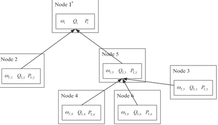
Figure 3.The message processing of the variables among intelligent nodes.
Figure2gives an example of constructing a BFS tree for a network with 6 nodes (controllers for 6 pumps connected in parallel). From the root node 1, the search message indicated by red links gradually spreads to leaf nodes. Based on the BFS tree, every node performs an algorithm enabling coordinations with its neighbors.
Below is a description of the main procedure in Algorithm1. Every node obtains its node type in the BFS tree (as root node, intermediate node, or leaf node). Then every node initializes its pump performance parameters, the range of speed ratio, the sample adjustment parameterτ, the child nodes setNiand the total iteration parameterK.
Every leaf node generates independently speed ratio samples following the uniform distribution
Algorithm 1:Breadth first search Random Sampling algorithm (BRS)
Input: the BFS tree, the pump parametersaP1,i,aP2,i,aP3,i,bP1,i,bP2,i,bP3,i, the total flow rateQ0, the headH0, sample
adjustment parameterτ, the child nodes setNi, the range of speed ratioω−andK; Output: every intelligent node’s optimal estimation of speed ratioωe
∗
i ; 1 ifnode is leaf node or intermediate nodethen
2 Initializek=0,QT,i,k−1= [],PT,i,k−1= [],ωT,i,k−1= [];
3 whiledoes not receive end instructiondo 4 Sampleωi,kandωi,k∼U[ω−−τ, 1];
5 ifωi,k≥ω−then
6 Use Equations (6)(7)(8) andH0to computeQi,k,Pi,k;
7 else
8 ωi,k=0,Qi,k=0,Pi,k=0 ;
9 DoAlgorithmA.2and getQT,i,k,PT,i,k,ωT,i,k;
10 ifQT,i,k≥Q0then
11 DeleteQT,i,k,PT,i,k,ωT,i,k;
12 k=k+1 ;
13 Send end instruction andωe
∗
kto child nodes ; 14 Goto final ;
15 ifnode is root nodethen 16 Initializek=0,Pk∗=∞,ωe
∗
k= [],QT,i,k−1= [],PT,i,k−1= [],ωT,i,k−1= [];
17 whilek<Kdo
18 Qi,k= [],Pi,k= [],ωi,k= [];
19 DoAlgorithmA.2and getQT,i,k,PT,i,k,ωT,i,k;
20 Qi,k=Q0−QT,i,k;
21 Use Equations (6)(7)(8) andH0to computeωi,k,ωT,i,k,PT,i,k;
22 ifPT,i,k<Pk∗then
23 ωe∗k=ωT,i,k,Pk∗=PT,i,k;
24 k=k+1 ;
25 Send end instruction andωe
∗
kto child nodes ; 26 Goto final ;
27 final;
28 returnits speed ratioωe
∗
i;
over the interval[ω−−τ, 1]withωi,kas the k-th sample of nodei. If the speed ratio sampleωi,k≥ω−, it will evaluate correspondingQi,k,Pi,k. If not, the node will set the sample to 0, which means the
pump will be shut down. Then the node will transmit theQT,i,k,PT,i,k,ωT,i,kto its parent node. If it
does not receive end instruction, the leaf node will continue to do the above operation. When the leaf node receives end instruction from the parent, it will stop generating samples, and acquire its optimal speed ratio. The intermediate node performs the same operation that generates samples. The difference is that the intermediate node will calculate the partial summation flow rateQT,i,kand the
partial summation power consumption PT,i,k over the subtree of nodeibasing on theQT,j,kj,PT,j,kj
provided by its child nodesNi. TheQT,j,kj,PT,j,kj is read from the input message queue. Next, if the
partial summation flow rateQT,i,k ≤Q0, the intermediate node will transmitQT,i,k,PT,i,k,ωT,i,kto its
parent node. If not, the node will delete theQT,i,k,PT,i,k,ωT,i,k. As for the root node, it will compute its
Qi,kthrough the total flow rateQ0and theQT,j,kj provided by its child nodes. This operation makes
sure that the constraint is satisfied. In view of theQi, the root node utilizes the Equations (6)(7)(8) and
H0to computeωi,k. Whenωi,ksatisfies the speed ratio range constraint, it will calculate the total energy
consumptionPT,i,k.Pk∗is the currently optimal total energy consumption afterkrounds selection of
speed ratio samples.ωe ∗
kdenotes the optimal estimation combination of speed ratio samples in thek-th
round for the root node. In addition, ifPT,i,k≤ Pk∗, the root node will updatePk∗andωe ∗
k to save the
rounds the root node supposes that the best combination of speed ratios is achieved, and therefore ends the entire algorithm and sends the best combination of speed ratiosωe
∗
kto child nodes. Once the
node receives the end message andωe ∗
k, it will stop calculation and send them to child nodes.
From the steps of Algorithm1, we can observe that BRS algorithm makes sure the solution exactly meets the demand (the total flow rate constraint). Every node maintains its own speed ratioωe
∗ i. The
whole adjustment is an iterative optimization process with the cooperation of each node. Constraints are satisfied in the entire iteration process. Besides, it has the flexibility due to the distributed control structure. We will prove that the total energy consumption can be minimized.
5. Theoretical analysis of the proposed algorithm
We carry out a theoretical analysis of the convergence for the proposed BRS algorithm. According to the definition of the algorithm, the sample process at nodei(for pump i) of speed ratio can be viewed as an i.i.d. stochastic process{ωi,k,k=1, 2, ...}whereωi,kis the k-th sample of the speed ratio
of pump i. The speed ratio sample of pump i follows the uniform distribution
U[ω−−τ, 1] (13)
withτ>0 as a given parameter such thatω− >τ.
Assumption 2. Both the energy consumption function Pi(ωi)and flow rate function Qi(ωi)of a pump are
continuous functions on the domain{0} ∪[ω−−τ, 1]with Pi(0) =Qi(0) =0. The flow rate function Qi(ωi)
of a pump is also a monotonously increasing function.
Now we are ready to show the main theoretical result: the speed ratios of the m pumps output by our BRS algorithm will converge to the optimal solution of the PSROP problem (defined in Section 3.2by Equations ((9)-(12)) if K goes to infinity. According to the steps of BRS algorithm, under Assumption1, all pump nodes are divided into three types on the spanning treeT. DenoteI as the set of intermediate nodes,Las the set of leaf nodes,R={r}as the set of single root node. Then we can rewrite PSROP in an equivalent form.
[Problem 2. Alternative Pump Speed Ratio Optimization Problem (PSROP’)]
min
ωi,i∈L∪I ∪{r}i∈L∪I ∪{
∑
r}Pi(ωi) (14)
s.t. H0=Hi i∈ L ∪ I ∪ {r} (15)
Q0=
∑
i∈L∪I ∪{r}
Qi (16)
ω−≤ωi≤1orωi =0, i∈ L ∪ I ∪ {r} (17)
It is trivial that the optimal value of PSROP’ is the same as that of PSROP since both objective functions and constraints are the same when we re-order the speed ratios. Below, in order to present our analysis, we define the optimal pump speed ratios according to node types of the spanning treeTas follows
ω∗T= [ω∗i,i∈ L ∪ I ∪ {r}] (18)
Similarly, we denote
ωT = [ωi,i∈ L ∪ I ∪ {r}] (19)
as the combination list of decision variables for PSROP’ problem and
e
ω∗T,K= [ωe ∗
as the speed ratios of the m pumps output by our BRS algorithm afterKrounds to emphasis the role of node type on the treeT. We note that due to the equality constraint Equation (16), the optimal speed ratioωr∗of the root nodercan be written as a function of speed ratios of other nodes. In fact, we have (due to the monotone property of flow rate function by Assumption2)
ωr∗=Qr−1(Q0−
∑
i∈L∪IQi(ωi∗)) (21)
Similarly, we have
e
ω∗r,K=Q−r 1(Q0−
∑
i∈L∪IQi(ωe ∗
i,K)) (22)
according to the step in Line 20 of Algorithm1running at the root node.
Assumption 3. ω∗r ∈(ω−, 1)and∑i∈L∪IQi(ω∗i)>0.
Theorem 1. Suppose Assumptions1,2,3are satisfied. Letε>0be any given positive number, then lim
K→∞Pr{|P(ωe ∗
T,K)−P(ωT∗)|<ε}=1 (23)
whereωe ∗ T,K= [ωe
∗
i,K,i∈ L ∪ I ∪ {r}]are speed ratios output by the algorithm after K rounds.
Proof of Theorem 1. From Assumption3, we know thatωr∗ ∈ (ω−, 1)and∑i∈L∪IQi(ω∗i) > 0. In this case, we know thatQr(ω∗r)>0 and∃i0∈ L ∪ Isuch that
Qi0(ω
∗
i)>0 (24)
We must haveQr(ω∗r)∈[Qr(ω−),Q0)andQi0(ω
∗
i0)∈(0,Q0)
Since bothQr andPrare continuous (by Assumption2), for anyε1 >0, there exists aδr(ε1) ∈ (0, 1−ω−)such that∀ωr∈[ωr−(ε1),ωr∗], whereωr−(ε1) =ω∗r −δr(ε1). It is true that
Qr(ωr)∈(Qr(ωr∗)−ε1,Qr(ω∗r)] (25)
Pr(ωr)∈(Pr(ω∗r)−ε1,Pr(ωr∗) +ε1) (26) Similarly, since bothQiandPiare continuous (by Assumption2), whenQi(ω∗i)>0(thenω∗i ∈ [ω−, 1]), for anyε2>0, there exists aδi(ε2)∈(0, 1−ω−)such that∀ωi∈Bi= [ω∗i,ω+i (ε2)],
Bi= [ωi∗,ωi+(ε2)] (27)
andωi+(ε2) =ω∗i +δi(ε2), it is true that
Q(ωi)∈[Qi(ωi∗),Qi(ωi∗) +ε2) (28) Pi(ωi)∈(Pi(ωi∗)−ε2,Pi(ω∗i) +ε2) (29) Whenω∗i =0, thenQi(ωi∗) =0, we setBi={0}. For this case,∀ωi∈Bi, Equations (28) and (29) still
hold.
Since the optimal solution is feasible, we have
Q0=Qr(ω∗r) +
∑
i∈L∪IQi(ωi∗) (30)
For a givenε1>0 and correspondingδr(ε1), we chooseε2in Equations (28) and (29) such that
or equivalently
∑
i∈L∪IQi(ωi∗) + (m−1)ε2≤Q0−Qr(ω−r (ε1)) (32)
For(ωi,i∈ L ∪ I)satisfying∩i∈L∪IBi, we have
ωr=Q−r 1(Q0−
∑
i∈L∪IQi(ωi)) (33)
ωr=Q−r 1(Qr(ω∗r) +
∑
i∈L∪I(Qi(ωi∗)−Qi(ωi)))≥Qr−1(Qr(ω∗r)−(m−1)ε2) (34)
ωr ≥Qr−1(Qr(ωr−(ε1))) = ω−r (ε1) (35) From the monotone property of Q−r 1(based on the monotone property of flow rate function by
Assumption2), we also have
ωr ≤Q−r1(Qr(ωr∗)) =ω∗r (36) So
ωr ∈[ωr−(ε1),ω∗r] (37)
From Equation (29) andPi(ωi)is set to 0 ifωi=0, we know that
∑
i∈L∪I
|Pi(ωi)−Pi(ω∗i)|<(m−1)ε2 (38)
Due to Equation (27), forωr in Equation (33) we have
Pr(ωr)∈(Pr(ω∗r)−ε1,Pr(ωr∗) +ε1) (39) In sum, we have
|
∑
i∈L∪I ∪{r}
Pi(ωi)−P(ω∗)|=|
∑
i∈L∪I ∪{r}(Pi(ωi)−P(ω∗i))|<Qr(ωr∗)−Qr(ωr−(ε1)) +ε1 (40)
For givenε>0, we can chooseε1such that
Qr(ω∗r)−Qr(ωr−(ε1)) +ε1<ε (41) For nodesi∈ L ∪ I, defineAi,kas the event that thekth sampleωi,kgenerated at nodeibelongs to
the intervalBidefined in Equation (27) with the understanding thatBi ={0}ifωi,k=0 (corresponding
to the caseui,k ∈[ω−−τ,ω−). According to the algorithm design, we have
Pr{Ai,k}=Pr{ωi,k ∈Bi}=
ω+i −ω∗i
1−(ω−−τ) (42)
ifQi(ωi∗)>0, or
Pr{Ai,k}=Pr{ωi,k ∈Bi}=Pr{ui,k∈[ω−−τ,ω−)}=
τ
1−(ω−−τ) (43)
ifQi(ω∗i) =0, it means the pump will be shut down. Since the samples generated at different nodes in
L ∪ Iare independent, we have
Pr{ \
i∈L∪I
Ai,k}=
∏
i∈L∪I
Pr{Ai,k} ≥[
d 1−(ω−−τ)]
wheredis a constant no large thanτand(ω+i −ω∗i)for nodesi∈ L ∪ Isuch thatQi(ω∗i)>0. From Equation (32), we know that ifωi,k∈ Bi,∀i∈ L ∪ I, it is true that
∑
i∈L∪IQi(ωi,k)<Q0 (45)
As a result,ωT,k= [ωi,k,i∈ L ∪ I;ωr,k]where
ωr,k=Q−r 1(Q0−
∑
i∈L∪IQi(ωi,k)) (46)
forms a feasible solution with total energy consumption as
P(ωT,k) =
∑
i∈L∪I ∪rPi(ωi,k) (47)
From the selection ofωe ∗
T,kas the feasible solution with the lowest total energy consumption for the
firstk-th rounds, we have
P(ωe∗T,k)≤P(ωT,k) (48)
From the optimality ofω∗and Equation (40), we have
P(ω∗)≤P(ωe ∗
T,k)≤P(ωT,k)≤P(ω∗) +ε (49) The theorem is proved.
As a result, BRS algorithm can not only exactly meet the constraints and have great flexibility but also has the guarantee of convergence. By applying BRS algorithm, the solutionωe
∗
T,kconverges to the
optimal speed ratioω∗in probability. Hence, under Assumption1, BRS algorithm is easy to realize and can converge to the optimal solution.
Remark: In reality, we cannot judge whether Assumption3holds in advance. To make sure the convergence to the global true optimal solution, we can run the algorithm with each node as the root node in turn and compare the final results.
6. Results and discussion
In this section, we will verify the properties of the proposed BRS algorithm including the demand satisfaction, minimum energy consumption, the flexibility in adapting to changing topology of pump systems and low-cost hardware test. We compare BRS with other methods in demand satisfaction and energy consumption. This section is organized as follows: First, we introduce the study cases, the simulation environment and compared algorithms. Second, we study the violation of constraint satisfaction among BRS and the compared algorithms. Third, we compare the performance among BRS and other algorithms. Then, we study the flexibility of BRS under a different number of intelligent nodes. Finally, we test BRS based on low-cost hardware.
6.1. Set up of study cases
10 20 30 40 50 60 70
Q (L/s)
30 35 40 45 50 55 60
H (m)
PUMP-B PUMP-A
10 20 30 40 50 60 70
Q (L/s)
0.5 0.6 0.7 0.8 0.9 1
PUMP-B PUMP-A
Figure 4.The performance curves of PUMP-A and PUMP-B
Table 2.Performance parameters of pumps.
Pump Performance Parameters
aP1,i aP2,i aP3,i bP1,i bP2,i bP3,i
PUMP-A -0.0046 0.0696 60.271 -0.0002 0.0254 0.0616 PUMP-B -0.0112 0.1358 54.841 -0.0005 0.0316 0.2582
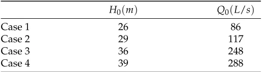
Table 3.Different demand of HVAC system.
H0(m) Q0(L/s)
Case 1 26 86
Case 2 29 117
Case 3 36 248
Case 4 39 288
Here, we establish an HVAC system including 6 pumps in parallel. 4 of pumps are PUMP-A (big pump) and 2 of pumps are PUMP-B (small pump). We adopt four different total flow rate and head demand cases in an HVAC system which represent the typical stable working conditions during a period of time as shown in Table3. These cases are from light to heavy. In order to investigate a method in depth, the optimal working positions for parallel pumps are different under these four cases.
6.2. Software simulation environment
The software simulation environment is as follows: The centralized algorithms SC, SLSQP and GA are built with Python to carry out the simulation. We employ the distributed simulation platform (DSP)1to investigate the performance of both BRS and TA. The operating environment is Win10x64, Intel (R) Core (TM) i7-7700 @3.60GHz, DSP1.0, and computer memory is 8 GB. Based on the DSP, we can simulate a distributed pump system to test BRS and TA algorithms under different HVAC system demand. DSP can generate different kinds of topologies for intelligent nodes. TA is designed under controllers connected in the chain topology and relaxes the constraint. If the topology changes, TA cannot obtain the violation of constraints. All nodes are connected one by one for distributed methods
1 DSP is a simulation engine written in python that can simulate distributed algorithms synchronous all nodes through UDP
in Section6.4. In Section6.6, we adopt a tree topology. The population size and iterations are the same for GA and BRS.
6.3. Algorithms to compare
The compared algorithms include centralized algorithms and distributed algorithm. We pick up three typical centralized algorithms including sequence control strategy (SC)[12], sequential least squares programming algorithm (SLSQP) [25] and genetic algorithm (GA) [23]. The distributed transfer algorithm (TA) was proposed in [26]. These algorithms are selected based on previous literature review. They are well represented characteristics of four class methods and show good performance. The details of these algorithms can refer to the related literatures.
6.4. The violation of constraint satisfaction
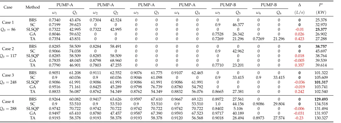
Table4presents the calculation results for five algorithms listed in Section6.3and for four cases listed in Section6.1.∆represents the violation of constraint (11), which means that∆=∑Qi−Q0.
The total flow rate exceeds the actual demand if∆is positive. The total flow rate is less than the actual demand if∆is negative. From Table4,∆related to BRS and SC are all 0 in the four cases and there are no violations to meet the constraint. As can be seen,∆for other three algorithms are positive or negative.
The reason for the performance difference among algorithms in constraint satisfaction for pump systems is that their principles are different. Our BRS algorithm and SC deal with the equality constraint directly. BRS algorithm uses the advantage of population sampling and the equality constraint to find feasible solutions. SC adopts the PID feedback control to eliminate the deviation and meet the constraint. The other three methods relax the equality constraint and adopt the penalty function. They cannot meet the constraint. Regardless of cases,∆is distributed randomly.
Experimental results prove that most methods have some violations to meet the demand. Furthermore, data comparison of∆confirms that our BRS algorithm can exactly satisfy the demand constraints, which is difficult to most methods.
Table 4.Numerical comparison for different study cases.
Case Method PUMP-A PUMP-A PUMP-A PUMP-A PUMP-B PUMP-B ∆ P
∗
ω1 Q1 ω2 Q2 ω3 Q3 ω4 Q4 ω5 Q5 ω6 Q6 (L/s) (KW)
Case 1 BRS 0.7340 43.476 0.7304 42.524 0 0 0 0 0 0 0 0 0 25.378
Q0=86
SC 0.7199 39.623 0 0 0 0 0 0 0.9 46.377 0 0 0 32.970
SLSQP 0.7322 42.995 0.7322 42.995 0 0 0 0 0 0 0 0 -0.01 25.377
GA 0.8046 59.632 0 0 0 0 0 0 0.7528 26.342 0 0 0.026 26.902
TA 0.7354 43.831 0 0 0 0 0 0 0.7269 21.296 0.7269 21.296 0.423 27.288
Case 2 BRS 0.8285 58.509 0.8284 58.491 0 0 0 0 0 0 0 0 0 38.757
Q0=117
SC 0.9066 74.038 0 0 0 0 0 0 0.9 42.962 0 0 0 45.697
SLSQP 0.8285 58.509 0.8285 58.509 0 0 0 0 0 0 0 0 0.018 38.764
GA 0.7835 48.045 0.8798 68.960 0 0 0 0 0 0 0 0 -0.005 39.539
TA 0.7790 46.901 0.7803 47.255 0 0 0 0 0.7710 23.201 0 0 0.357 39.614
Case 3 BRS 0.9051 61.208 0.9111 62.552 0.9076 61.775 0.9107 62.465 0 0 0 0 0 101.322
Q0=248
SC 0.9 60.036 0.9 60.036 0.9046 61.098 0 0 0.9 33.415 0.9 33.415 0 105.609
SLSQP 0.9086 61.991 0.9086 61.991 0.9086 61.991 0.9086 61.991 0 0 0 0 -0.036 101.317
GA 0.9516 71.161 0.8425 45.289 0.9798 76.739 0.8780 54.792 0 0 0 0 -0.019 103.741
TA 0.8833 56.087 0.8762 54.349 0.8762 54.349 0.8832 56.076 0.8665 27.381 0 0 0.242 102.540
Case 4 BRS 0.9264 60.082 0.9417 63.626 0.9597 67.610 0.9667 69.121 0.8972 27.561 0 0 0 129.493
Q0=288
SC 0.9 53.510 0.9 53.510 0.9 53.510 0.9 53.510 1.0 44.156 0.9086 29.804 0 134.518
SLSQP 0.9742 70.722 0.9742 70.722 0.9742 70.722 0.9742 70.722 0.8402 5.106 0 0 -0.006 131.494
GA 0.9497 65.410 0.8780 47.457 0.9587 67.390 0.9593 67.523 0.9717 40.189 0 0 -0.031 131.937
TA 0.9193 58.378 0.9193 58.378 0.9193 58.378 0.9120 56.568 0.9018 28.494 0.8973 27.574 -0.23 130.327
6.5. Performance comparison
291
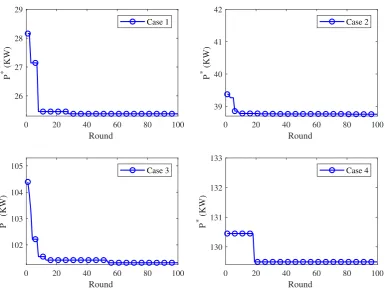
consumption. When comparingP∗of BRS to that of SC in the four cases, it is clear that the energy consumption of BRS is the minimum to exactly meet the demand constraint. ComparingP∗among BRS and other three algorithms in the four cases, the energy consumption of BRS is the minimum in Case 2 and Case 4. The energy consumption of SLSQP is slightly lower than BRS in Case 1 and Case 3. The reason is that the solutions of SLSQP are not feasible and the total flow rate is less than the actual demand. Due to providing less flow rate, the energy consumption of SLSQP is minimum. The differences ofP∗between SLSQP and BRS are 0.001 and 0.005 in Case 1 and Case 3. Table4shows that SC can satisfy the demand constraint. But SC does not optimize the energy consumption and pumps work in the non-optimal points. As a result, SC consumes much more energy.
According to these findings, due to lacking the guarantee of convergence, these methods cannot work optimally in most cases. Our BRS algorithm makes sure to satisfy the demand and minimize the energy consumption of pumps. It consumes less energy in the four cases and verifies the guarantee of convergence.
From Table4, it can be observed that there are different combinations of pumps for type PUMP-A and type PUMP-B in the four proposed cases. In Case 1, we can choose the first option to open two PUMP-A, the second option to open one PUMP-A and two PUMP-B or the third option to open one PUMP-A and one PUMP-B. BRS algorithm makes sure to satisfy the demand and have a minimum energy consumption. The combination of pumps with BRS is supposed to be optimal.
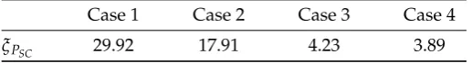
Table4shows that only BRS and SC can exactly meet the demand constraints. SC is wildly used in practical engineering. In order to show the energy saving potential between two algorithms, we define the energy saving rateξPas follows. WherePiSCis the energy consumption of pumpiunder SC.
PiBRSis the energy consumption of pumpiunder BRS.
ξPSC =
∑PiSC−∑PiBRS
∑PiBRS ×100% (50)
Table 5.The energy saving rate for different cases.
Case 1 Case 2 Case 3 Case 4
ξPSC 29.92 17.91 4.23 3.89
Table5summarizes the energy save rate of pumps in the four cases under different algorithms, clearly showing that BRS is more energy efficient than SC. During the four work cases, the maximum energy saving of BRS is about 29.92%, which indicates that BRS can save more energy in practical engineering. This energy saving ability reflects that BRS has a great ability to find good enough solutions.
0 20 40 60 80 100
Round
26 27 28 29
P
* (KW)
Case 1
0 20 40 60 80 100
Round
39 40 41 42
P
* (KW)
Case 2
0 20 40 60 80 100
Round
102 103 104 105
P
* (KW)
Case 3
0 20 40 60 80 100
Round
130 131 132 133
P
* (KW)
Case 4
Figure 5.The iteration of BRS under four cases.
6.6. Test of flexibility
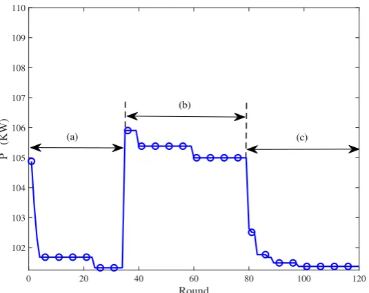
The testing scenario is as follows: First, all nodes work well as shown in Figure6(a). Then, Node 4 PUMP-A breaks down or is in maintenance as shown in Figure6(b). Next, Node 4 is repaired as shown in Figure6(c). The total flow rate and head demand on the main pipe is Case 3 listed in Section 6.1.
2
5
4
6
3
*
1
2
5
4
6
3
*
1
2
5
4
6
3
(a) (b) (c)
*
1
0 20 40 60 80 100 120
Round
102 103 104 105 106 107 108 109 110
P
* (KW)
(a) (c)
(b)
Figure 7.The iteration of BRS under different number of nodes.
Figure7shows the iteration process of BRS under different number of nodes corresponding to the ones in Figure6. From Figure7,P∗tends to converge to the optimal points. When all pumps work well as shown in Figure6(a)(c),P∗converges to the same optimal point. As expected, the number of nodes changing does not hinder the capacity of our algorithm to cooperate with neighbors and perform the on-line optimization. BRS algorithm does not need to stop the whole pump system and the pump is plug-and-play. In contrast, the centralized control methods need to explicitly reformulate the problem to be solved manually and hard to automate in practice.
These experiments validate that our BRS algorithm can adapt to the system dynamic changing by reallocating the flow rates in an on-line fashion.
6.7. Hardware test of BRS
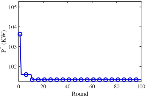
Furthermore, we developed a distributed low-cost hardware platform to test the algorithm performance. The hardware platform is based on Raspberry Pi3, Model B, 1GB RAM. Every Raspberry Pi3 represents an intelligent node and has the wireless and Ethernet communication interface. It can connect with neighbor nodes through wireless communication interface. Every node stores the pump model and simulates a smart pump. Figure8presents the topology of the pump nodes. The total flow rate and head demand on the main pipe is Case 3 listed in Section6.1.
1
2
3
4 5
6 3
0 20 40 60 80 100 Round
102 103 104 105
P
* (KW)
Figure 9.The iteration of BRS on hardare platform.
Figure9shows the iteration process of BRS algorithm on the hardware platform. BRS algorithm can converge to the optimal point in the first few iterations, which clearly shows that BRS algorithm can perform on Raspberry Pi3-based low-cost hardware platform. The whole hardware system is fully distributed and there are not any central monitoring hosts. When the number of pumps increases, traditional centralized methods need a high-cost computing platform to perform the centralized optimization. As a result, BRS algorithm can reduce the system cost.
7. Conclusions
The distributed optimization problem with parallel-connected pumps is studied in this paper. We propose a distributed optimal control algorithm BRS for on-off status and flow rates of parallel-connected pumps in HVAC systems. The proposed BRS algorithm consists of two parts: First, in order to process the network information, we apply the breadth first search algorithm to construct a tree for exchanging messages. Second, all nodes coordinate with each other and randomly sample the speed ratios. The intelligent nodes communicate with their neighboring nodes and run collaboratively to perform the proposed distributed approach. Compared with existing methods, the solutions of our BRS algorithm meet the total flow rate demand without any deviations and achieve the minimum pump energy consumption. BRS algorithm has the convergence guarantee and shows the great flexibility in adapting to the system dynamic changing.
The methodology and its advantages are demonstrated through a numerical example. Besides, we show that the BRS algorithm works on low-cost hardware. As a future work, we will try to extend the algorithm to asynchronous networks. If the condition is allowed, we will test BRS algorithm in practical systems.
Author Contributions:All authors make contributions to the research of this paper. X.W. wrote the manuscript. Q.Z. revised the findings of this work. Y.W. developed the distributed simulation platform.
Funding: This work was supported by National Key Research and Development Project of China (No. 2017YFC0704100 entitled New generation intelligent building platform techniques, and 2016YFB0901900) and the National Natural Science Foundation of China (No. 61425027), the 111 International Collaboration Program of China under Grant BP2018006 and the BNRist Program under Grant No. BNR2019TD01009.
Conflicts of Interest:The authors declare no conflict of interest.
aP1,i,aP2,i,aP3,i,bP1,i,bP2,i,bP3,i pump performance parameters
Hi head of pumpi(m)
H0 total head demand(m)
m total number of pumps
ni actual speed of pumpi
n0,i rated speed of pumpi
Ni set of child nodes of nodei
Pk∗ optimal estimation of total power consumption after thek-th sample
Pi power consumption of pumpi
PT,i,k partial summation power consumption over subtree of nodei
QT,i,k partial summation flow rate over subtree of nodei
Qi flow rate of pumpi(L/s)
Q0 total flow rate demand(L/s)
RT,i,δ combination of node’s optimal speed ratio neighborhood over the subtree of nodei Greek letters
ωi speed ratio of nodei
ω− lower limitation of speed ratio
ωi,k thek-th speed ratio sample of nodei
ωT,i,k the combination of the speed ratio over subtree of nodei
ωi∗ optimal speed ratio
e
ωi,k∗ optimal estimation of speed ratio after thek-th sample
ω∗ optimal combination of speed ratio
e
ω∗k optimal estimation combination of speed ratio after thek-th sample
ξP energy saving rate
ηi mechanical efficiency
ηM,i motor efficiency
ηVFD,i variable frequency efficiency
∆ violation of∑Qi−Q0
Subscripts
i pumpi
k thek-th sample
T the subtree
Appendix A
Appendix A.1
Algorithm 2:Breadth First Search algorithm [33] Input: Choose one nodeias a root
Output: Every node appoint a parent variable to convey its parent
1 Initialize:isends search message to neighbors ; 2 ifan unmarked node accepts messagethen
3 Mark itself;
4 Appoint one node that sends search to it as parent;
5 Send search to neighbors at next step ; 6 Goto final;
7 final;
Appendix A.2
Algorithm 3:Message processing algorithm
Input: the child nodes setNi, the flow rateQi,k, the power consumptionPi,k, the speed ratioωi,k, QT,i,k−1,PT,i,k−1,ωT,i,k−1;
Output: every intelligent node’s the partial summation flow rateQT,i,k,the partial summation power consumption PT,i,kand the combination of the speed ratioωT,i,kover subtree of nodei;
1 InitializeQT,i,k=Qi,k,PT,i,k=Pi,k,ωT,i,k= [ωT,i,k,ωi,k];
2 SendQT,i,k−1,PT,i,k−1,ωT,i,k−1message to parent’s input message queue and receive child nodej,j∈ Nimessage ;
3 QT,i,k=QT,i,k+∑j∈N
iQT,j,kj;
4 PT,i,k=PT,i,k+∑j∈NiPT,j,kj;
5 ωT,i,k= [ωT,i,k, S
j∈Ni
ωT,j,kj];
6 returnQT,i,k,PT,i,k,ωT,i,k;
Abbreviations
The following abbreviations are used in this manuscript:
HVAC Heating, ventilating, and air-conditioning system BRS Breadth first search random sampling algorithm BFS Breadth first search algorithm
SC Sequence control strategy
SLSQP Sequential least squares programming algorithm
GA Genetic algorithm
TA Transfer algorithm
DSP Distributed simulation platform
References
1. Pérez-Lombard, L.; Ortiz, J.; Pout, C. A review on buildings energy consumption information.Energy Build
2008, 40, 394—398.
2. Arun Shankar, VK.; Umashankar, S.; Paramasivam, S.; Hanigovszki, N. A comprehensive review on energy efficiency enhancement initiatives in centrifugal pumping system.Appl Energy2016, 181, 495–513.
3. Liu, M.; Ooka, R.; Choi, W.; Ikeda, S. Experimental and numerical investigation of energy saving potential of centralized and decentralized pumping systems.Appl Energy2019, 251:113359.
4. Kusiak, A.; Li, M.; Tang, F. Modeling and optimization of HVAC energy consumption.Appl Energy2010, 87, 3092–102.
5. Ali, A.; Coté, C.; Heidarinejad, M.; Stephens, Brent. Elemental: An Open-Source Wireless Hardware and Software Platform for Building Energy and Indoor Environmental Monitoring and Control.Sensors2019, 19. 4017.
6. Zhao, Q.; Wang, X.; Wang, Y.; Jiang, Z.; Dai, Y. A P2P Algorithm for Energy Saving of a Parallel-Connected Pumps System. In: Fang Q., Zhu Q., Qiao F. (eds) Advancements in Smart City and Intelligent Building. ICSCIB2018. Advances in Intelligent Systems and Computing, vol 890, 385-395.Springer, Singapore. 7. Zhao, Q.; Jiang, Z. Insect Intelligent Building (I2B): A New Architecture of Building Control Systems Based
on Internet of Things (IoT). In: Fang Q., Zhu Q., Qiao F. (eds) Advancements in Smart City and Intelligent Building. ICSCIB2018. Advances in Intelligent Systems and Computing, vol 890, 457-466. Springer, Singapore.
8. Wang, S.; Burnett, J. Online adaptive control for optimizing variable-speed pumps of indirect water-cooled chilling systems.Appl. Therm. Eng.2001, 21, 1083-1103.
9. Li, H.; Shi, J.; Li, Z.; Yang, C.; Zhang, Y.; Liang, Z. A Group Control Method of Central Air-conditioning Chilled Water Pumps with the Aim of Energy Saving. 2018 Int Conf Power Syst Technol POWERCON 2018 -Proc 2019:4517–24. https://doi.org/10.1109/POWERCON.2018.8602089.
10. Tianyi, Z.; Liangdong, M.; Jili, Z. An optimal differential pressure reset strategy based on the most unfavorable thermodynamic loop on-line identification for a variable water flow air conditioning system.
11. Ma, Z.; Wang, S. Energy efficient control of variable speed pumps in complex building central air-conditioning systems.Energy Build2009, 41, 197–205.
12. Gao, D.C.; Wang, S.; Sun, Y. A fault-tolerant and energy efficient control strategy for primary-secondary chilled water systems in buildings.Energy Build2011, 43, 3646–56.
13. Bonvin, G.; Demassey, S.; Le Pape, C.; Maïzi, N.; Mazauric, V.; Samperio, A. A convex mathematical program for pump scheduling in a class of branched water networks.Appl Energy2017, 185, 1702–11.
14. Horváth, K.; van Esch, B.; Vreeken, D.; Pothof, I.; Baayen, J. Convex Modeling of Pumps in Order to Optimize Their Energy Use. Water Resour Res2019, 55, 2432–45.
15. Koor, M.; Vassiljev, A.; Koppel, T. Optimization of pump efficiencies with different
pumps characteristics working in parallel mode. Adv Eng Softw 2016, 101, 69–76.
https://doi.org/10.1016/j.advengsoft.2015.10.010.
16. Menke, R.; Abraham, E.; Stoianov, I. Modeling Variable Speed Pumps for Optimal Pump Scheduling[C]// World Environmental and Water Resources Congress 2016.2016.
17. Jepsen, K.L.; Hansen, L.; Mai, C.; Yang, Z. Power consumption optimization for multiple parallel centrifugal pumps. 1st Annu IEEE Conf Control Technol Appl CCTA 2017 2017;2017-January:806–11.
18. Wang, J.Y.; Chang, T.P.; Chen, J.S. An enhanced genetic algorithm for bi-objective pump scheduling in water supply. Expert Syst Appl2009, 36, 10249–58. https://doi.org/10.1016/j.eswa.2009.01.054.
19. Rong, Z.G.; W, T.Y. Global optimization of pump configuration problem using extended crowding genetic algorithm.Chinese Journal of Mechanical Engineering.2004;17:1.
20. Cimorelli, L.; Covelli, C.; Molino, B. Optimal Regulation of Pumping Station in Water Distribution Networks Using Constant and Variable Speed Pumps: A Technical and Economical Comparison. Energies,2020, 13: 2530.
21. Barán, B.; Von, Lücken C.; Sotelo, A. Multi-objective pump scheduling optimization using evolutionary strategies. Adv Eng Softw 2005;36:39–47. https://doi.org/10.1016/j.advengsoft.2004.03.012.
22. Hashemi, SS.; Tabesh, M.; Ataeekia, B. Ant-colony optimization of pumping schedule to minimize the energy cost using variable-speed pumps in water distribution networks. Urban Water J2014, 11, 335–47.
23. Olszewski, P. Genetic optimization and experimental verification of complex parallel pumping station with centrifugal pumps.Appl Energy2016, 178, 527–39.
24. Liu, Z.; Chen, X.; Xu, X.; Guan, X. A decentralized optimization method for energy saving of HVAC systems. IEEE Int Conf Autom Sci Eng 2013:225–30. https://doi.org/10.1109/CoASE.2013.6654019.
25. Kraft, D. A software package for sequential quadratic programming. Forschungsbericht- Deutsche Forschungs- und Versuchsanstalt fur Luft- und Raumfahrt,1988.
26. Dai, Y.; Jiang, Z.; Shen, Q.; Chen, P.; Wang, S.; Jiang, Y. A decentralized algorithm for optimal distribution in HVAC systems.Build Environ2016, 95, 21–31.
27. Beckerle, P.; Schaede, H.; Rinderknecht, S. Fault Diagnosis and State Detection in Centrifugal Pumps—A Review of Applications. Mech Mach Sci 2015;21. doi:10.1007/978-3-319-06590-8.
28. Zheng, W.; Wu, W.; Zhang, B.; Li, Z.; Liu, Y. Fully distributed multi-area economic dispatch method for active distribution networks. IET Gener Transm Distrib2015, 9, 1341–51.
29. Timotheou, S.; Panayiotou, CG.; Polycarpou, MM. Distributed Traffic Signal Control Using the Cell Transmission Model via the Alternating Direction Method of Multipliers. IEEE Trans Intell Transp Syst2015, 16, 919–33.
30. Campana, PE.; Li, H.; Yan, J. Dynamic modelling of a PV pumping system with special consideration on water demand.Appl Energy2013, 112, 635–45.
31. Pumps S. Centrifugal Pump Handbook (Third Edition). Elsevier Science,2010.
32. Ulanicki, B.; Kahler, J.; Coulbeck, B. Modeling the efficiency and power characteristics of a pump group.J. Water Resour. Plan. Manage.-ASCE2008, 134, 88-93.
33. Lynch, NA. Distributed algorithms. Elsevier,1996.