Article
Multi-Temporal Crop Type and Field Boundary
Classification with Google Earth Engine
Michael Lukas Marszalek 1,*, Maximilian Lösch 1, Marco Körner 2 and Urs Schmidhalter 1
1 Chair of Plant Nutrition, Technical University of Munich, Emil-Ramann-Straße 2, 85354 Freising, Germany;
[email protected]; [email protected]
2 Chair of Remote Sensing Technology, Technical University of Munich, Arcisstraße 21, 80333 München,
Germany; [email protected]
* Correspondence: [email protected]; Tel.: +49-8161-71-3739
Abstract: Crop type and field boundary mapping enable cost-efficient crop management on the field scale and serve as the basis for yield forecasts. Our study uses a data set with crop types and
corresponding field borders from the federal state of Bavaria, Germany, as documented by farmers from 2016 to 2018. The study classified corn, winter wheat, barley, sugar beet, potato, and rapeseed
as the main crops grown in Upper Bavaria. Corresponding Sentinel-2 data sets include the normalised difference vegetation index (NDVI) and raw band data from 2016 to 2018 for each
selected field. The influences of clouds, raw bands, and NDVI on crop type classification are analysed, and the classification algorithms, i.e., support vector machine (SVM) and random forest (RF), are compared. Field boundary detection and extraction are based on non-iterative clustering
and a newly developed procedure based on Canny edge detection. The results emphasise the
application of Sentinel’s raw bands (B1–B12) and RF, which outperforms SVM with an accuracy of
up to 94%. Furthermore, we forecast data for an unknown year, which slightly reduces the classification accuracy. The results demonstrate the usefulness of the proof-of-concept and its
readiness for use in real applications.
Keywords: Precision farming; Crop type mapping; Digital agriculture; Sentinel-2; Random Forest; SVM; Field boundaries; Canny; Simple non-iterative clustering
1.Introduction 1.1.Motivation
Agricultural productivity needs to be increased and its environmental impact must be reduced to meet the future demand for food and achieve sustainable development goals (SDGs). Precision
farming covers various technological aspects, including satellite data, drone applications, machine learning, navigation, and communication, with a focus on supporting farmers and healthy
environment to achieve sustainability, climate-related goals, and profitability. Plants can thus get the right amount of water, fertilisers, and pesticides and reach optimal yields while the use of resources
and environmental impact are decreased. In addition to providing spatial information, precision farming supports the temporal requirement and helps farmers optimise the irrigation or fertilisation
of crops.
Crop type classification is a goal of this research and entails the detection of crop types in unknown areas without a priori information. The detection of agricultural areas gives suppliers,
policy makers, and governments an up-to-date overview of areas under crops and their potential yields. Remote sensing provides multispectral data and especially since the launch of the Sentinel mission, the amount of data has been continuously increasing. With its various satellites and sensors,
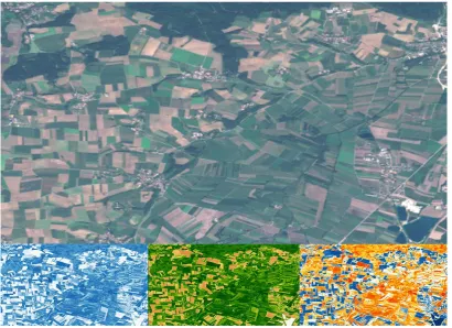
the Sentinel mission enables innovative applications in different domains, such as agriculture or geology. Figure 1 presents a sample red-green-blue (RGB) image of Sentinel-2 with three different
multispectral visualisations. The spatial and temporal resolutions are suitable for precision agriculture and its applications. In this study, we analyse the usability of the indices and raw bands
of Sentinel-2 for crop type and field boundary mapping. A detailed comparison with current research activities is provided in Section 1.2. This publication additionally presents the methods chosen and
an in-depth overview of the necessary steps to generate field borders or classify crop types.
Figure 1. Sentinel-2 in RGB and its multispectral indices, which deliver various important growth and health information for every crop type. The visualised area is one of our experimental areas in the scope of this research.
1.2.State of the art
Since 2018, less impact has been observed owing to the nominal 5-day revisit cycle [3]. Data from the Moderate Resolution Imaging Spectroradiometer (MODIS) are generally used to forecast yields at the county level but do not fulfil the spatial resolution requirement of precision farming. Convolutional neural networks have shown excellent results with MODIS data. Crop type mapping is usually based on radar or optical data from Sentinel-1 or Sentinel-2, respectively. Some researchers fused both data sets and attained a maximum accuracy of 82% [4]. The authors state that a combination of Sentinel-1 and Sentinel-2 data outperforms approaches based on either radar or optical measurements alone [4]. Bargiel et al. [5] analysed phenological sequence patterns with Sentinel-1 and attained F1 scores of 0.74–0.79. Rußwurm et al. [6,7] experimented with long short-term memory neural nets and Sentinel-2 raw bands as input data, attaining an overall accuracy (OA) of up to 89.7%. Saini et al. [8] tested single-date images from Sentinel-2 using support vector machines (SVMs) and Random Forest (RF) in the Roorkee district of India. The results showed that the OAs of the classifications achieved by RF and SVM using Sentinel-2 imagery were 84.22% and 81.85%, respectively [8]. Immitzer et al. [9] confirmed the high values of the red-edge and shortwave infrared (SWIR) bands for vegetation mapping but the usage of these raw bands additionally improved the classification tasks in comparison with those achieved by single index-based classification studies. Dimitrov et al. [10] too used Sentinel-2 as training data to apply sub-pixel classification to PROBA images with a resolution of 100 m/pixel. The chosen machine learning methods, i.e., SVM and RF, provided classification accuracies ranging from 67% for grasslands to 92% for broad-leaved forests. Random forest performed better than maximum likelihood or SVM classifiers with OA in the range 73–93% [11]. Random forest, artificial neural networks, and SVMs have been compared in several publications for crop type mapping [12,13] but the effect of input data or predictions for future years based on past observed values have rarely been addressed.
In general, both object-based and pixel-based classification approaches are detailed in the literature with an emphasis on the advantages of the former. For instance, an object-based approach was adopted in a previous work [14] with accuracies in the range 78.1–96.2%. Blaschke et al. [15] mentioned that object-based approaches use image segmentation to identify regions with similar characteristics of homogeneity, which reduces feature space and computation time compared with those achieved by pixel-based approaches [15]. There exist several examples of unmanned aerial vehicle-based classification with high-resolution data [16,17]. Herein, RF achieved accuracies of up to 94.6% through object-based classification. While much research has focused on the mapping of crop species, the mapping of field boundaries seems to be a niche problem. However, it represents an important feature of yield prediction on the field scale, especially for regions without official field boundary data. National authorities can usually accomplish this with inputs from farmers. A satellite-based approach can automate this time-consuming procedure and track boundary changes over time. Contour detection and segmentation with high-resolution images obtained from WorldView data were analysed by Marshall et al. [18]. The results showed that both methods were not suitable for challenging areas. While segmentation seemed to lead to over-segmentation, contour detection performed better in the case of fields larger than 0.01 square kilometre. Masoud et al. [19] proposed an approach based on convolutional networks, providing field boundaries and scaling up the resolution from 10 m/pixel to 5 m/pixel. A comparison with RapidEye images, which had an original resolution of 5 m/pixel, showed only minor differences. A convolutional neural network with only one composite image as the input was additionally verified [20].
1.3.Overview
for classification. Most publications focus on one or more indices, such as normalised difference vegetation index (NDVI) (Figure 2). The SWIR bands, B11 and B12, exhibit important properties and hence, we include all the bands and compare the results with those obtained using NDVI. Additionally, simple non-iterative clustering (SNIC) and our own index-based Canny edge procedure for field boundary extraction are introduced. While SNIC is a standard Google Earth Engine algorithm for the clustering of similar pixels, our approach benefits from the uniform colour distribution of the normalised difference water index (NDWI), its emphasised edges, and a compilation of several Canny edge images across the vegetation period. Our data set differs from those used in previous studies regarding the number of fields and temporal distribution. The data set extends from 2016 until 2018 and is also applied to the forecast for 2018, based on a model with data from 2016 and 2017. Time series forecasts dramatically influence the OA because of weather anomalies. The semantic segmentation of significant features, which are weather-independent to the extent possible, can boost classification accuracies and provide a stable classification for unknown regions and years.
Section 1 provides a general introduction including our motivation, state-of-the-art activities, and our goals. Section 2 gives a detailed description of our data set and study site, as well as the methods used such that an interested reader can replicate our work. The results are presented in Section 3, which additionally shows the various experiments and corresponding accuracies. The discussion and conclusions in Sections 4 and 5, respectively, complete this research work and entail proposals for further investigations.
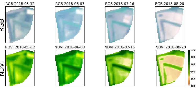
Figure 2. Example for a time series data set of a field with four RGB and NDVI samples during the vegetation period 2018. NDVI is a relative index providing leaf chlorophyll content information and related information, such as biomass, plant health or nitrogen.
2.Materials and Methods 2.1.Study site
The study site is Upper Bavaria in Southern Germany with about 7875 square kilometre of agricultural land and an average field size of 0.02 km2[22]. The main crop types are corn, winter wheat, barley, rapeseed, sugar beet, and potato. Of these, corn, winter wheat, and barley are the predominant crops. Bavaria has an annual average temperature of 8.6 °C and average precipitation of 811 mm. Figure 3 shows the typical crop periods with the sowing and harvest months. Figure 4
illustrates the average maximum and minimum temperatures, monthly precipitation, and all the agricultural areas from OpenStreetMap (OSM). We focused on the vegetation period 2016–2018. The
manifest in 2018, which reduced yields by approximately 10%. This weather anomaly affected crop type mapping, especially in 2018, because of the unfavourable climatic conditions.
Figure 3. Crop phenology of crop types considered. Sowing is marked in lime, green stands for the vegetation period, and yellow covers the harvest period in Bavaria.
Figure 4. Climate overview of Upper Bavaria and a photo of the Alps. Figure a) shows all the agricultural areas
from OSM in EPSG:4326. Figure b) shows Upper Bavaria and Bavaria as an overlay in EPSG:3857.
2.2.Crop data
Our crop type data set, provided by the Bavarian State Ministry of Agriculture and Forestry (StMELF), acts as the basis for the development of the crop type classification and field boundary detection methods. This data set includes crop types with field borders for 2016, 2017, and 2018. The
study focuses on Upper Bavaria and the crops considered are corn, winter wheat, barley, sugar beet, potato, rapeseed, and an additional rejection class called ‘Other’, which covers all other crops, such
as grassland and summer barley. Crop Type
Corn
Winter wheat Winter barley Winter rapeseed Potato
Sugar beat
Sowing Growth Harvest
Dez
2.3.Sentinel-2
The Sentinel-2 mission, with its two twin satellites Sentinel-2A and Sentinel-2B, monitors the Earth with a resolution of up to 10 m/pixel and a revisit time of 2–5 days depending on latitude. The availability of useful data is nevertheless limited due to clouds. Each identical satellite is equipped with a multispectral sensor, that covers 13 spectral bands and has a swath width of 290 km. Sentinel-2A was launched in June 2015 followed by Sentinel-2B in March 2017. Sentinel-2 provides visible and near-infrared (NIR) spectral bands (B2, B3, B4, B8) with a resolution of 10 m/pixel and SWIR bands (B11, B12) with a resolution of 20 m/pixel. Band 1 is for aerosol, while bands 9 and 10 are suitable for detecting water vapour and cirrus clouds. These bands provide a resolution of 60 m/pixel for atmospheric corrections and do not need higher resolutions. Table 1 summarises the properties. In this study, Sentinel’s Level 1C product was downloaded from Google Earth Engine, which stores terabytes of up-to-date satellite data and provides an efficient and fast way to access this information through a JavaScript or Python interface [23,24]. The time series data includes raw bands and indices for each test field and year from 2016 to 2018.
Table 1: Overview of bands of Sentinel-2 [23]
Sentinel-2 Bands Central Wavelength (nm) Resolution (m) Description
Band 1 443.9 (S2A) /
442.3 (S2B) 60
Aerosol
Band 2 496.6 (S2A) /
492.1 (S2B) 10
Blue
Band 3 560 (S2A) /
559 (S2B) 10
Green
Band 4 664.5 (S2A) /
665 (S2B) 10
Red
Band 5 703.9 (S2A) /
703.8 (S2B) 20
Red Edge
Band 6 740.2 (S2A) /
739.1 (S2B) 20
Red Edge
Band 7 782.5 (S2A) /
779.7 (S2B) 20
Red Edge
Band 8 835.1 (S2A) /
833 (S2B) 10
NIR
Band 8A 864.8 (S2A) /
864 (S2B) 20
NIR
Band 9 945 (S2A) /
943.2 (S2B) 60
Water vapour
Band 10 1373.5 (S2A) / 1376.9 (S2B) 60
Cirrus
Band 11 1613.7 (S2A) / 1610.4 (S2B) 20
SWIR
Band 12 2202.4 (S2A) / 2185.7 (S2B) 20
SWIR
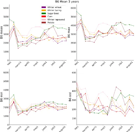
decided to focus on Level 1C products based on the assumption that it is appropriate for our case study and is consistent with our data set, which includes data from 2016 onwards. In contrast, Google Earth Engine provides Level 2A images starting from 2017. We plotted the min, max, standard deviation, and mean for every band to determine a significant feature differentiating crop types.
Figure 5. Reflection differences using band 6 and its mean, min, max and standard deviation as mean.
Figure 5 and Figure 6 show band 6, band 12, and the temporal trend for every crop type.
Especially, band 12 (SWIR) allows the detection of marked differences. Time, as a feature, uncovers crop type differences as well. Mean values separate crop types very well and are used as model inputs in our experiments. Our indices include water- and chlorophyll-based indices, which provide
information on leaf water content and biomass, respectively, for each field. We computed every index using Google Earth Engine and downloaded all the results into a corresponding file for further
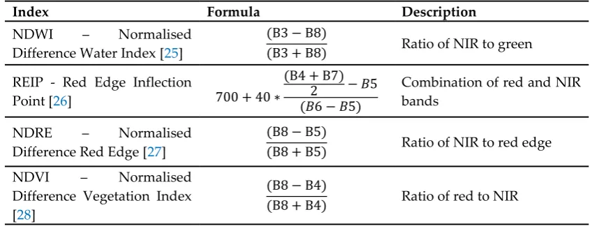
analysis. Table 2 summarizes all the indices used and their characteristics. The NDVI is frequently used to monitor biomass or plant health. It is the most common index used in research activities for
yield predictions or crop type classification. The use of NDVI showed better performance than that achieved with normalised difference red edge (NDRE) or red edge inflection point (REIP), and hence,
Figure 6. Reflection differences using band 12 (SWIR). The various crop types show different reflection
properties over time.
Table 2: Indices and corresponding characteristics
Index Formula Description
NDWI – Normalised
Difference Water Index [25]
(B3 − B8)
(B3 + B8) Ratio of NIR to green
REIP - Red Edge Inflection
Point [26] 700 + 40 ∗
(B4 + B7) 2 − 𝐵5 (𝐵6 − 𝐵5)
Combination of red and NIR bands
NDRE – Normalised
Difference Red Edge [27]
(B8 − B5)
(B8 + B5) Ratio of NIR to red edge
NDVI – Normalised
Difference Vegetation Index [28]
(B8 − B4)
The NDWI shows very good results for field boundary detection. It visualises water content better and does not reveal spatial differences to the extent revealed by an RGB or NDVI image. Fewer
irrelevant Canny edges reduce noise and improve performance; this is presented in Section 3.1. All the experiments are based on the raw bands (B1-B12) and mean NDVI mean values as input for crop type classification. All the fields in our data set are randomly selected and include 2099 agriculture
fields and the corresponding time series data from Sentinel-2. The satellite data consist of mean values for each field and date and were downloaded from Google Earth Engine using a cloud meta filter of
20%. The CLOUDY_PIXEL_PERCENTAGE parameter considers cloudy pixels for a Sentinel-2 scene but does not recognise all cloudy pixels on the field scale. Some applications, such as field borders
detection, need a completely cloud-free images, and hence we propose an alternative solution in Section 2.4. The crop type detection method can handle the small amount of noise introduced by
cloudy pixels.
Figure 7.Visualization of NDVI trends for all crop types. NDVI mean, NDVI min, NDVI max and NDVI
2.4.Clouds and interpolation
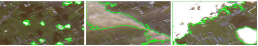
Figure 8. Cloud detection based on OpenCV
Several cloud detection techniques were evaluated with a focus on fast processing time. For instance, bands 10 and 11 were excellent candidates for cloud detection and were used in our data set. However, they did not guarantee a completely cloud-free time series. Sentinel-Hub [29] implemented a Python framework, that detects clouds in Sentinel-2 images at the expense of processing time. We designed an alternative approach using OpenCV and its contour detection. Figure 8 showsthree sample images with clouds detected in them. Our OpenCV-based cloud filtering takes RGB images as the input and rejects images in which clouds are detected such that a maximised cloud-free image collection serves as the input for field boundary detection. Clouds introduce noise and falsify the resultant boundaries. In contrast, crop type mapping was accomplished with a cloud cover property of 20% for every scene.
Another important task of the study is temporal interpolation. Working with time series data entails several problems, such as gaps, different time steps, and noisy measurements. Lepot et all. [30] reviewed interpolation methods, such as nearest-neighbour and linear interpolation. Sentinel images are available every 3 to 5 days for our study sites but cloud coverage reduces the amount of suitable data, which needs to be re-sampled and interpolated. To cover the phenological development, we decided upon a 2-weeks resolution of our time series data. Figure 9 shows an example of raw Sentinel-2 measurements over time in comparison with cloud-filtered and interpolated measurements for the same field and year. The maxima in the left shows clouds with high reflectance values. Polynomial interpolation performs slightly better, but does not approximate the real reflectance values when satellite data are not available for the beginning of the vegetation period. Linear interpolation shows stable performance in all the cases and is, therefore, used.
2.5.SVMs and RF
Machine learning includes unsupervised, supervised, and reinforcement-learning models in order to analyse, classify, and predict trends. Unsupervised learning provides a set of algorithms, which uncover insights without additional labels. On the contrary, supervised learning uses labels such that a target output is associated with various predictors. Reinforcement learning models entail agents, environment, and corresponding interactions in order to maximise rewards. A detailed description of this approach can be found in the literature [31] but is not in the focus of the present work. Supervised learning ,with its methods of SVM and RF for classification analysis, are used for crop type classification in this work.
Support vector machines can perform linear and non-linear classification tasks and regression analysis. Non-linear classification especially uses a kernel, that maps an input space to a high-dimensional feature space. An input set is separated into classes or categories with a clear, maximised gap between these categories. Every training sample consists of an assigned class (output) and its observations (input). A theoretical description and overview can be found in the literature [32,33]. Random Forest performs classification and regression tasks as well [34]. It is an interesting approach that comprises several almost uncorrelated decision trees, each of which is trained by a random subset of the training data set with substitution (bootstrapping). Individual decision trees tend to overfit but a combination of several uncorrelated trees overcomes this issue. Each decision tree provides a class prediction, but the final result is obtained from the aggregation of all the predictions by averaging the outputs. Both algorithms are part of the machine learning Python library scikit-learn, which is used in this research.
2.6.Classification accuracy
The performance evaluation of crop type mapping is based on overall accuracy (OA), producer’s accuracy (PA), user’s accuracy (UA) and Kappa statistics. The PA and UA values are presented for each crop type while the OA and Kappa values evaluate the global performance of our trained model. All the metrics are part of scikit-learn too. The OA represents the number of correctly classified crops divided by all the reference crops. The Kappa coefficient is a measure in the range 0–1 and quantifies prediction and ground truth. For instance, a value of 1 indicates a perfect match between the prediction and ground truth. The PA shows how well a classification matches with the ground truth while the UA refers to the reliability of the classification. A description of the metrics and examples can be found in the literature [35]. Cross-validation (CV) has also been applied to avoid over-fitting and is based on the cross_val_score of Scikit-learn.
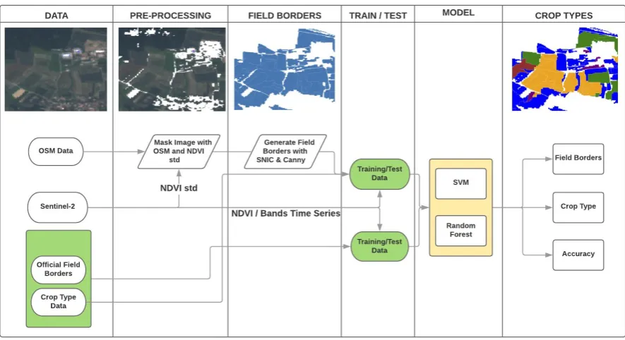
2.7.Overview of processing
Figure 10. General overview of the processing chain with its data as input, processing steps, and models
2.8.Field boundaries
Especially for regions without field border information, field mapping is an important step towards yield forecasts and crop type mapping. We implemented three procedures, compared the resultant polygons visually, and applied them to a challenging area with narrow fields (12). The first algorithm, SNIC, used all the bands of Sentinel-2 as input. As the SNIC over-segments an image and produces many irrelevant boundaries, we decided to introduce a novel approach based on Canny, an algorithm for detecting edges in images. Further information on Canny and SNIC can be found in the literature [36,37]. This procedure additionally includes cloud detection, as introduced in Section
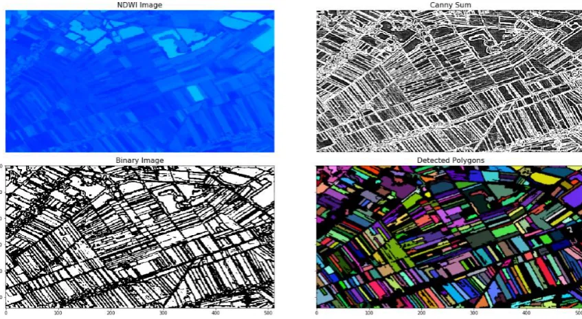
2.4. Adding all the Canny results over a period of time improves boundary detection. Figure 11 shows the processing pipeline with its OpenCV processing steps and geo-referenced polygons as the output.
Figure 11: Field boundary detection with OpenCV and Google Earth Engine
3.Results
3.1.Field boundary detection
polygons detected. The final output was additionally masked with OSM data in order to clear roads, buildings, and lakes, which were detected as polygons. Small fields (<0.2 𝑚2) or artefacts were filtered for the generation of Figure 14. The RGB-based Canny edge uncovers fewer details than the NDWI does. The SNIC over-segments the area and does not show clear boundaries. We applied bicubic resampling to smooth our image collection and could thus slightly improve the boundary visualisation. The resolution of 10 m/pixel is a limiting factor; nonetheless, it still provides good results. The application of bands with lower resolutions, such as B6 or B7, should therefore be avoided. Nevertheless, the field boundary pipeline can be further improved, for instance with higher resolutions or improvements in the processing pipeline. The processing of the images introduced small gaps between the fields, which can be resolved by slightly increasing the polygon size.
Figure 12. RGB-based detection of field boundaries with OpenCV
Figure 14. Comparison of resultant geo-referenced polygons
3.2.Crop type classification
Table 3: Confusion matrix for SVM with NDVI. All ground truth data for every crop type are summarised under
‘Total’ in the last row of the confusion matrix. Total of classified crops is presented in the column ‘Total’.
Other Winter wheat (WW) Winter barley (WB) Winter rapeseed (WR)
Corn Potato Sugar beet (SB)
Total UA (%)
PA (%)
Other 61 7 4 10 2 2 0 86 70.93 67.78
WW 6 59 4 7 0 0 0 76 77.63 71.95
WB 8 4 53 12 0 0 0 77 68.83 77.94
WR 6 10 6 32 0 0 0 54 59.26 51.61
Corn 7 1 1 1 43 12 8 73 58.90 69.35
Potato 0 1 0 0 7 59 1 68 86.76 68.60
SB 2 0 0 0 10 13 66 91 72.53 88.00
Total 90 82 68 62 62 86 75 525
OA 71% Kappa 0.85 CV 0.67
Table 4: Confusion matrix for SVM with all bands
Other Winter wheat (WW) Winter barley (WB) Winter rapeseed (WR)
Corn Potato Sugar beet (SB)
Total UA (%)
PA (%)
Other 62 5 5 0 6 4 1 83 74.70 83.78
WW 3 66 2 1 1 0 0 73 90.41 82.50
WB 2 6 74 4 0 0 0 86 86.05 90.24
WR 2 2 0 67 4 1 0 76 88.16 93.06
Corn 1 1 0 0 57 3 0 62 91.94 79.17
Potato 4 0 0 0 3 63 3 73 86.30 87.50
SB 0 0 1 0 1 1 69 72 95.83 94.52
Total 74 80 82 72 72 72 73 525
Table 5: Confusion matrix for RF with NDVI. All ground truth data for every crop type are summarised under
‘Total’ in the last row of the confusion matrix. Total of classified crops is presented in the column ‘Total’.
Other Winter wheat (WW) Winter barley (WB) Winter rapeseed (WR)
Corn Potato Sugar beet (SB)
Total UA (%)
PA (%)
Other 60 1 1 4 1 2 0 69 86.96 76.92
WW 3 59 7 8 1 0 0 78 75.64 82.51
WB 3 3 75 4 0 0 0 85 88.24 84.27
WR 5 3 4 45 0 0 0 57 78.95 72.58
Corn 4 2 1 1 53 7 13 81 65.43 80.30
Potato 3 1 1 0 4 61 4 74 82.43 78.21
SB 0 0 0 0 7 8 66 81 81.48 79.52
Total 78 69 89 62 66 78 83 525
OA 80% Kappa 0.88 CV 0.71
Table 6: Confusion matrix for RF with all bands
Other Winter wheat (WW) Winter barley (WB) Winter rapeseed (WR)
Corn Potato Sugar beet (SB)
Total UA (%)
PA (%)
Other 65 1 0 0 1 1 0 68 95.59 85.53
WW 4 64 3 0 0 0 0 71 90.14 86.49
WB 4 5 69 2 0 0 0 80 86.25 94.52
WR 1 2 1 67 0 0 0 71 94.37 97.10
Corn 1 2 0 0 62 3 1 69 89.86 95.38
Potato 1 0 0 0 2 70 3 76 92.11 90.91
SB 0 0 0 0 0 3 87 90 96.67 95.60
Total 76 74 73 69 65 77 91 525
Table 7: Confusion matrix for RF with all bands and without class ‘Other’
Winter wheat (WW)
Winter barley (WB)
Winter rapeseed
(WR)
Corn Potato Sugar beet (SB)
Total UA (%)
PA (%)
WW 64 5 0 1 0 0 70 91.43 85.33
WB 8 71 0 1 0 0 80 88.75 92.21
WR 1 1 71 0 0 0 73 97.26 100.0
Corn 2 0 0 55 3 0 60 91.67 91.67
Potato 0 0 0 2 77 1 80 96.25 92.77
SB 0 0 0 1 3 83 87 95.40 98.81
Total 75 77 71 60 83 84 450
OA 94% Kappa 0.98 CV 0.9
The trained model, presented in Table 6, was applied to a location near Dürnast and for the year 2018. The training data set does not include this area, and this allows us to test the performance of our model in a real world scenario. Figure 16 shows the recorded results from StMELF which act as ground truth data, followed by the classification results. The OA is 80% which is lower than expected, considering the results in Table 6. In another experiment the same model was applied on the same area but without the additional class 'Other’, leading to an accuracy of 96%. Figure 17 shows the classification without the class ‘Other’. The model experiences difficulties in differentiating among winter wheat, winter rapeseed and winter barley. The class ‘Other’ includes various types of crops, such as different types of grasslands, summer barley, and soybean. It introduces an error, especially in regions with crops not covered in our model. Table 7 confirms the performance without the class ‘Other’. The performance of this model is very promising and is analysed in terms of feature importance (Figure 15). It reveals that the bands B3, B4, B5, B6, B7, B8, B8A, B11, and B12 are the most important features, especially in May and August.
Figure 16. Crop classification based on RF and all bands for an area near Dürnast in 2018. The first image shows
the recorded crop types (ground truth data) while the second image shows the classified crop types. The last
Figure 17. Crop classification based on RF and all bands without the class ‘Other’. The first image shows the
recorded crop types (ground truth data) while the second image shows the classified crop types. The last image
3.3.Time series and prediction for an unknown year
The time series prediction was analysed to develop a system for detecting crop types without data for the year considered. Figure 18 shows the raw reflectance values for band B6 and the crop types considered in our study.
Figure 18. Comparison of B6_mean reflectance across years
The reflectance values are influenced by weather conditions and the growth progress. Nevertheless, the trend remains comparable across years, and a separation between crops is given as well. We trained a model with data from 2016 and 2017 and forecast values for 2018. The OA was 77% with a Kappa of 0.89 (see Table 8). The growing season of 2018 was dry and showed an overall decrease in yield, which influenced the spectral response. Weather anomalies influence the accuracy of yield forecasts but do not have a comparable effect on the classification of crops. In another
experiment, the class ‘Other’ was excluded and the model was trained with our six crop types and
data from 2016 and 2017. Furthermore, the test data for 2018 did not include the class ‘Other’. Table
Table 8: Confusion matrix for RF with all bands based on a model trained with data for 2016 and 2017
Other Winter wheat (WW) Winter barley (WB) Winter rapeseed (WR)
Corn Potato Sugar beet (SB)
Total UA (%)
PA (%)
Other 77 10 16 2 7 1 0 113 68.14 77.0
WW 8 76 15 4 0 0 0 103 73.79 76.0
WB 5 12 63 2 0 0 0 82 76.83 63.0
WR 2 0 6 92 0 0 0 100 92.00 92.0
Corn 3 0 0 0 67 1 0 71 94.37 67.0
Potato 5 2 0 0 25 98 34 164 59.76 98.0
SB 0 0 0 0 1 0 66 67 98.51 66.0
Total 100 100 100 100 100 100 100 525
OA 77% Kappa 0.89 CV 0.89
Table 9: Confusion matrix for RF with all bands and without class ‘Other’
Winter wheat (WW) Winter barley (WB) Winter rapeseed (WR)
Corn Potato Sugar beet (SB)
Total UA (%)
PA (%)
WW 95 28 8 1 0 0 132 71.97 95.0
WB 3 67 2 1 0 0 73 91.78 67.0
WR 0 3 90 0 0 0 93 96.77 90.0
Corn 0 1 0 63 1 0 65 96.92 63.0
Potato 2 1 0 34 99 27 163 60.74 99.0
SB 0 0 0 1 0 73 74 98.65 73.0
Total 100 100 100 100 100 100 525
Figure 20. Forecast for 2018 using a model trained with data for 2016 and 2017 and without class ‘Other’,
4.Discussion
The results obtained and the experimental approaches used for field boundary detection show the influence of input data on the performance. Data cleaning and preparation are very important
steps to be carried out at the beginning of every data science project. Crop type mapping too benefits from the type of input and its configuration. Segmentation of images has been studied in several
works but its adaption to Earth observation has rarely been carried out. Gorelick [36] experimented with SNIC and other approaches. We experienced over-segmentation with SNIC and tested Canny
with RGB and NDWI images. The NDWI-based Canny edge detection showed very good results, which can be further improved. Using only RGB bands (B2, B3, B4) appeared to be a good step initially, as changes in RGB images over time are discernible to the human eye as well. In fact, the use
of RGB bands introduced a high number of edges, many of which were irrelevant and not just field boundaries. This noise even reduced the number of polygons detected eventually. The NDWI maps
leaf moisture or water content in general with a more simply distributed visualisation. This actually represents a benefit. It does not introduce many edges and focuses on field boundaries or object
boundaries in general. The results show that even small fields can be detected using the NDWI-based approach. Crop type mapping was evaluated using all the raw bands and NDVI. Indices, such as
NDRE or NDWI, did not perform better in the separation of crops, and hence, we focused on NDVI in this work. A more detailed analysis can be found in the literature [38], which acts as a precedent for the present research. In the previous work, the influence of interpolation, NDWI and NDRE were
additionally compared. The additional rejection class ‘Other’ for further plant types, such as grassland, reduced the classification accuracies in our experiment. The application of raw bands
outperformed the use of a single index. Especially, the bands B6, B7, B8, B11, or B12 have a significant impact on the results. An additional success factor is pre-processing, which includes cloud filtering,
interpolation type, and data cleaning. Nevertheless, clouds do not influence crop type mapping as much as they impact field boundary detection. Linear interpolation is a good choice for many use
cases. Polynomial interpolation approximates a time series more accurately but introduces errors, especially for data sets with several gaps in the beginning of the vegetation period. Filtering an image
collection with OSM data is recommended. It reduces the amount of data and focuses on agricultural areas. The presented results confirm very good classification accuracies. The model explains the variations in our data set very well. In contrast, forecasting a future data set (for instance, 2018)
remains a challenging step and entails decreased accuracies. The weather in 2018 was exceptionally dry and our model did not reflect this anomaly but provided very good results. We propose to
evaluate approximately weather-independent features, such as crop colour or height, in future works. These features are additionally affected by weather conditions but possibly do not respond to
weather anomalies as much as raw band reflections do. Nevertheless, it should be stressed that the performance of our model is very good and renders it suitable for use in a real application. In other
research activities, radar-based data, e.g. from Sentinel-1, were used for the mapping of crop species. Getting data independent of cloud conditions can be advantageous in regions with high cloud
5.Conclusions
This study addressed several aspects of crop type mapping and field boundary detection. Both applications represent important steps towards yield mapping on the field scale, especially in regions
without additional information. We used RF and SVMs with their underlying configurations. Using our approach, we classified several crop types with very high precision. The NDWI-based field
boundary detection can be further improved and has the potential to automate a time-consuming and important task. Random forest outperforms SVMs in crop type mapping. Especially, the usage
of all raw bands uncovers additional information, which cannot be seen using a single index, such as NDVI, alone. Data cleaning, interpolation, and cloud filtering influence the final performance and are the most important and time-intensive work packages initially. The results show that our model
outperforms many proposed approaches. The crop types and agricultural fields detected can serve as the basis for near real-time yield predictions. Forecasting future values is a challenging task but
mandatory for real applications. Therefore, an experiment was conducted to forecast 2018 data using a model trained with 2016 and 2017 data. The accuracy declined owing to the unfavourable weather
conditions impacting plant growth and yield in 2018. The weather was hotter and drier in 2018 than in 2017 and 2016 and influenced our model reliability. These results emphasise the importance of
distinguishing between the results of random train/test splits and forecasts of a future data set. Crop type mapping and field boundary detection do not need an online or near real-time approach but yield forecasts on the field scale would benefit from such an approach. Nevertheless, this study shows
the efficiency and potential of Sentinel data for use in real-world applications. The Sentinel mission with its growing data set and advancements in machine learning will uncover new insights and can
contribute to a more sustainable world.
Author Contributions: M.L. developed the general approach in the scope of his Master thesis. ML is the author of the processing software with contributions by M.M. In general, the following contributions have been made: “conceptualization, M.L. and M.M.; methodology, M.L. and M.M.; software, M.L. and M.M.; validation, M.L. and M.M.; writing—original draft preparation, M.M.; writing—review and editing, M.M., M.L., M.K. and U.S.; project administration, U.S.; funding acquisition, U.S.
Funding: The research work was supported by funds of the Federal Ministry of Food and Agriculture (BMEL) based on a decision of the Parliament of the Federal Republic of Germany via the Federal Office for Agriculture and Food (BLE) under the innovation support program for the project 28-1-B3.030-16.
Acknowledgments: StMELF, the Bavarian State Ministry of Agriculture and Forestry supported this research with its crop type data set. The authors are thankful for this dataset, which was a key for the scope of this research. We also like to thank all colleagues, which contributed with valuable recommendations and improvements on this manuscript. Finally, we would like to acknowledge the work of ESA regarding its Sentinel mission, which will enable new applications.
Conflicts of Interest: The authors declare no conflict of interest. The funders had no role in the design of the study; in the collection, analyses, or interpretation of data; in the writing of the manuscript, or in the decision to publish the results. We requested a permission for the crop type dataset, which covers Bavaria. StMELF provides this dataset on request for selected research projects.
References
1. Bolton, D.K.; Friedl, M.A. Forecasting crop yield using remotely sensed vegetation indices and crop
phenology metrics. Agricultural and Forest Meteorology 2013, 173, 74–84, doi:10.1016/j.agrformet.2013.01.007.
2. El-Shirbeny, M.A.; Abutaleb, K. Sentinel-1 Radar Data Assessment to Estimate Crop Water Stress. WJET
3. Skakun, S.; Vermote, E.; Franch, B.; Roger, J.-C.; Kussul, N.; Ju, J.; Masek, J. Winter Wheat Yield Assessment
from Landsat 8 and Sentinel-2 Data: Incorporating Surface Reflectance, Through Phenological Fitting, into
Regression Yield Models. Remote Sensing 2019, 11, 1768, doi:10.3390/rs11151768.
4. van Tricht, K.; Gobin, A.; Gilliams, S.; Piccard, I. Synergistic Use of Radar 1 and Optical
Sentinel-2 Imagery for Crop Mapping: A Case Study for Belgium. Remote Sensing 2018, 10, 1642,
doi:10.3390/rs10101642.
5. Bargiel, D. A new method for crop classification combining time series of radar images and crop phenology
information. Remote Sensing of Environment 2017, 198, 369–383, doi:10.1016/j.rse.2017.06.022.
6. Rußwurm, M.; Lefèvre, S.; Körner, M. BreizhCrops: A Satellite Time Series Dataset for Crop Type
Identification, Time Series Workshop of the 36th International Conference on Machine Learning (ICML), Long
Beach, California, 2019. http://arxiv.org/pdf/1905.11893v1.
7. Rußwurm, M.; Körner, M. Multi-Temporal Land Cover Classification with Sequential Recurrent Encoders.
IJGI 2018, 7, 129, doi:10.3390/ijgi7040129.
8. Saini, R.; Ghosh, S.K. Crop Classification on Single Data Sentinel-2 Imagery using Random Forest and
Support Vector Machine. Int. Arch. Photogramm. Remote Sens. Spatial Inf. Sci. 2018, XLII-5, 683–688,
doi:10.5194/isprs-archives-XLII-5-683-2018.
9. Immitzer, M.; Vuolo, F.; Atzberger, C. First Experience with Sentinel-2 Data for Crop and Tree Species
Classifications in Central Europe. Remote Sensing 2016, 8, 166, doi:10.3390/rs8030166.
10. Dimitrov, P.; Dong, Q.; Eerens, H.; Gikov, A.; Filchev, L.; Roumenina, E.; Jelev, G. Sub-Pixel Crop Type
Classification Using PROBA-V 100 m NDVI Time Series and Reference Data from Sentinel-2 Classifications.
Remote Sensing 2019, 11, 1370, doi:10.3390/rs11111370.
11. Ray, S.S. Exploring Machine Learning Classification Algorithms for Crop Classification using Sentinel 2
Data. Int. Arch. Photogramm. Remote Sens. Spatial Inf. Sci. 2019, XLII-3/W6, 573–578,
doi:10.5194/isprs-archives-XLII-3-W6-573-2019.
12. Pandya, M., Baxi, A., Potdar, M.B., Kalubarme, M, H. and Agrawal, B. Comparison of Various Classification
Techniques for Satellite Data, International Journal of Scientific & Egineering Research, Vol. 4, Issue 2,
February-2013.
13. Nitze, I., Schulthess, U., Asche, H. Comparison Of Machine Learning Algorithms, Random Forest,
Artificial Neural Network And Support Vector Machine To Maximum Likelihood For Supervised Crop
Type Classification. GEOBIA 2012.
14. Belgiu, M.; Csillik, O. Sentinel-2 cropland mapping using pixel-based and object-based time-weighted
dynamic time warping analysis. Remote Sensing of Environment 2018, 204, 509–523,
doi:10.1016/j.rse.2017.10.005.
15. Blaschke, T. Object based image analysis for remote sensing. ISPRS Journal of Photogrammetry and Remote
Sensing 2010, 65, 2–16, doi:10.1016/j.isprsjprs.2009.06.004.
16. Böhler, J.; Schaepman, M.; Kneubühler, M. Crop Classification in a Heterogeneous Arable Landscape
Using Uncalibrated UAV Data. Remote Sensing 2018, 10, 1282, doi:10.3390/rs10081282.
17. Wei, L.; Yu, M.; Liang, Y.; Yuan, Z.; Huang, C.; Li, R.; Yu, Y. Precise Crop Classification Using
Spectral-Spatial-Location Fusion Based on Conditional Random Fields for UAV-Borne Hyperspectral Remote
Sensing Imagery. Remote Sensing 2019, 11, 2011, doi:10.3390/rs11172011.
18. Marshall, M.; Crommelinck, S.; Kohli, D.; Perger, C.; Yang, M.Y.; Ghosh, A.; Fritz, S.; Bie, K.d.; Nelson, A.
Landscapes of Ethiopia with Very High Spatial Resolution Imagery. Remote Sensing 2019, 11, 2082,
doi:10.3390/rs11182082.
19. Masoud, K.M.; Persello, C.; Tolpekin, V.A. Delineation of Agricultural Field Boundaries from Sentinel-2
Images Using a Novel Super-Resolution Contour Detector Based on Fully Convolutional Networks. Remote
Sensing 2020, 12, 59, doi:10.3390/rs12010059.
20. Waldner, F., Diakogiannis, F. Deep learning on edge: extracting field boundaries from satellite images with
a convolutional neural network, 2019. http://arxiv.org/pdf/1910.12023v1.
21. Inglada, J.; Arias, M.; Tardy, B.; Hagolle, O.; Valero, S.; Morin, D.; Dedieu, G.; Sepulcre, G.; Bontemps, S.;
Defourny, P.; et al. Assessment of an Operational System for Crop Type Map Production Using High
Temporal and Spatial Resolution Satellite Optical Imagery. Remote Sensing 2015, 7, 12356–12379,
doi:10.3390/rs70912356.
22. Bayerisches Landesamt für Statistik. Statistische Berichte - A5113 201700: Flächenerhebung n. Art d.
tatsächlichen Nutzung in Bayern zum Stichtag 31. Dezember 2017.
23. Google Earth Engine. Spectral Bands.
https://developers.google.com/earth-engine/datasets/catalog/COPERNICUS_S2 (accessed on 19
November 2019).
24. Gorelick, N.; Hancher, M.; Dixon, M.; Ilyushchenko, S.; Thau, D.; Moore, R. Google Earth Engine:
Planetary-scale geospatial analysis for everyone. Remote Sensing of Environment 2017, 202, 18–27,
doi:10.1016/j.rse.2017.06.031.
25. Gao. B.C., 1. NDWI - a normalized difference water index for remote sensing of vegetation liquid water
from space. Remote Sensing of Environment, 58, pp. 257-266.
26. Guyot, G., Baret, F., and Major, D.J. High spectral resolution: Determination of spectral shifts between the
red and infrared. International Archives of Photogrammetry and Remote Sensing, 11, pp. 750-760.
27. Barnes, E.M., Clarke, T.R., Richards, S. E., Colaizzi, P.D., Haberland, J., Kostrzewski, M., Waller, P., Choi,
C., Riley, E., Thompson, T., Lascano, R.J., Li, H., Moran, M.S. Coincident detection of crop water stress,
nitrogen status and canopy density using ground-based multispectral data. Proceedings of the Fifth
International International Conference on Precision Agriculture, Bloomington, MN, USA (Vol. 1619), July 2000.
28. Rouse, J.W, Haas, R.H., Scheel, J.A., and Deering, D.W. Monitoring Vegetation Systems in the Great Plains
with ERTS. Proceedings, 3rd Earth Resource Technology Satellite (ERTS) Symposium, vol. 1, p. 48-62.
29. Sentinel-Hub. Sentinel 2 cloud detector.
https://github.com/sentinel-hub/sentinel2-cloud-detector (accessed on May, 2019)
30. Lepot, M.; Aubin, J.-B.; Clemens, F. Interpolation in Time Series: An Introductive Overview of Existing
Methods, Their Performance Criteria and Uncertainty Assessment. Water 2017, 9, 796,
doi:10.3390/w9100796.
31. ROBOT LEARNING, edited by Jonathan H. Connell and Sridhar Mahadevan, Kluwer, Boston, 1993/1997,
xii+240 pp., ISBN 0-7923-9365-1 (Hardback, 218.00 Guilders, $120.00, £89.95). Robotica 1999, 17, 229–235,
doi:10.1017/S0263574799271172.
32. Cortes, C.; Vapnik, V. Support-vector networks. Mach Learn 1995, 20, 273–297, doi:10.1007/BF00994018.
33. Cristianini, N.; Shawe-Taylor, J. An introduction to support vector machines and other kernel-based
learning methods, 13. print; Cambridge Univ. Press: Cambridge, 2012, ISBN 9780521780193.
35. Humbold State University. GSP 2016 Introduction to Remote Sensing.
http://gis.humboldt.edu/OLM/Courses/GSP_216_Online/lesson6-2/metrics.html (accessed on 25 January
2020).
36. Gorelick, N. Segmentation.
https://docs.google.com/presentation/d/1p_W06MwdhRFZjkb7imYkuTchatY5nxb5aTRgh6qm2uU/view#
slide=id.p (accessed on 27 January 2020).
37. Chandwadkar, R., Dhole, S.P. Comparison of Edge Detection Techniques, 6th Annual Conference of IRAJ,
August, 2013, doi:10.13140/RG.2.1.5036.7123.
38. Maximilian Lösch. Maschinelles Lernen und Fruchtartenklassifizierung mittels multitemporaler
Fernerkundungsdaten. Masterarbeit; Technical University of Munich, Weihenstephan, Freising, 2019.

![Table 1: Overview of bands of Sentinel-2 [23]](https://thumb-us.123doks.com/thumbv2/123dok_us/8076923.1347511/6.595.137.459.305.717/table-overview-of-bands-of-sentinel.webp)