UNCERTAINTY PROPAGATION IN SEISMIC PROBABILISTIC RISK
ASSESSMENT
–
CASE STUDY
Alidad Hashemi1,2, Tarek Elkhoraibi1,3, and Farhang Ostadan1,4
1
Bechtel Earthquake Engineering Center
2
Senior Structural Engineer, Bechtel National, Inc., San Francisco, CA, USA, [email protected]
3
Senior Structural Engineer, Bechtel National, Inc., San Francisco, CA, USA
4
Bechtel Fellow, Bechtel National, Inc., San Francisco, CA, USA
ABSTRACT
The propagation of aleatory and epistemic uncertainties in calculation of seismic annual probability of failure is demonstrated for structural and non-structural limit state functions for a case study involving a typical nuclear facility structure on soil and rock sites. The uncertainties are accounted for in seismic hazard curves, geotechnical properties, structural properties and modelling, as well as structural and non-structural capacity parameters. The site uncertainties are propagated using probabilistic seismic hazard analysis (PSHA), 1-D probabilistic site response analysis (SRA) and probabilistic soil-structure interaction (P-SSI) analyses. The mean, median, and fractiles of the fragility curves are calculated for the selected limit state functions at 3 input intensity levels corresponding to ground motions with 104, 105, and 106 return periods which are deaggregated into their dominant low-frequency and high-frequency events. Using the median and fractiles of the fragility curves and surface hazard curves, the mean and logarithmic standard deviation of the annual probabilities of failure are calculated for the selected limit state functions. The proposed approach presents a rigorous example of seismic probabilistic risk assessment (SPRA) using probabilistic SSI analysis, as well as fragility curves and fractiles that are estimated at three points, representing three seismic intensity levels to illustrate the soil nonlinear effects at each level. The adequacy of the analysis sample size, the comparison between one-point and three-point fragility function estimations, and the relative importance of the seismic hazard and fragility uncertainties are also examined.
INTRODUCTION
The importance of seismic probabilistic risk assessment (SPRA) and probabilistic seismic hazard analysis (PSHA) in achieving the objectives of performance-based design, assessment of the realistic median capacity and response in order to make risk informed decision is well understood within the nuclear industry. The 2011 Fukushima earthquake and tsunami highlighted the need for comprehensive hazard and risk analysis for existing nuclear infrastructure worldwide. In the United States, the Nuclear Regulatory Commission (NRC) has mandated all existing nuclear power plants with updated ground motion exceeding the original design basis and review level earthquake to carry out a seismic margins assessment (SMA) or SPRA in the next few years. The NRC, the Nuclear Energy Institute (NEI), and the Electric Power Research Institute (EPRI) have developed guidelines and recommendations for such analysis for existing power plants (e.g. EPRI, 2013). The procedures currently proposed are yet to be completely tested in practice and may benefit from further refinement. The SPRA and PSHA can also be applied to other important structures and for locations outside of the United States to facilitate cost-benefit analyses of different design options or demonstrate the seismic resiliency the plants.
23rd Conference on Structural Mechanics in Reactor Technology Manchester, United Kingdom - August 10-14, 2015 Division VII
propagation of the soil and structural uncertainties through probabilistic site response analysis, probabilistic soil-structure interaction (SSI) analysis including probabilistic nonlinear interface and structural response to develop fragility curves for structural elements and non-structural important-to-safety (ITS) components. However, the previously presented methodology did not address the often significant uncertainty in the underlying seismological inputs used in PSHA.
The purpose of this paper is to complement the previously presented methodology and provide a consistent and rigorous approach for the fragility analysis and SPRA including the overall uncertainties in seismic hazard, geotechnical data, and structural properties through representative case studies. Special attention is given to the treatment of uncertainties, namely the distinction and separation of uncertainties into aleatory (random) variability and epistemic uncertainty, which allows for the calculation of mean as well as fractile fragility curves and annual probabilities of failure (PF). Other issues addressed in this paper are the assessment of the sample size, as well as a comparison with the scaling approach (also known as single point fragility estimation) in determination of the fragility curves, which is widely used in the nuclear industry today.
METHODOLOGY
The Integrated Soil-Structure Fragility Analysis (ISSFA) evaluates the seismic performance of a soil-structure system by quantifying its annual failure probability. The ISSFA methodology is intended to establish analysis techniques for developing a more reliable performance-based seismic design. The input data are the site specific seismic hazard curves (mean, median and fractiles) at surface or at bedrock level at depth, and soil dynamic properties, as well as the dynamic model of the subject systems, structures, and components (SSC). The output products are the fragility functions (mean, median and fractiles) for specified limit states that in conjunction with the hazard curves yield the annual probability of failure (performance) for the SSC and its corresponding uncertainty. A summary of the steps required for implementation of the ISSFA is presented below. Note that Steps 7 and 8 are performed only in the case where soil-structure interface non-linearity and/or structural non-linearity are explicitly considered.
1. Select the parameters and associated uncertainties in the dynamic system. Key variables include soil profiles described by their dynamic soil properties (e.g. shear wave velocity, Poisson’s ratio, unit weight, and soil degradation and damping curves), structural properties (e.g. concrete elastic modulus, structural damping, nonlinear models), soil structure interface properties (e.g. coefficient of friction for sliding). Each parameter is defined by a statistical distribution with a specified median (log-mean) and logarithmic standard deviation (log-SD). Proper consideration of aleatory variability and epistemic uncertainty for each parameter allows a rigorous definition of the fragility curves and their fractiles. Total number of independent parameters chosen is K.
2. Determine the necessary sample size N to represent the uncertainty in these variables, and generate a pseudo-random sample for each of the selected variables. Using Latin Hypercube Sampling (LHS, McKay et al. 1979), the variables are paired to form N sets, each comprised of K
randomized values for the K selected variables. A sample size of N=30 is selected for the case study in this paper. The adequacy of N is discussed later.
3. Determine the desired limit state functions based on realistic modes of failure. These limit state functions may include a subset of different failure events and scenarios. In the case study presented in this paper, the structural limit state function is defined in terms of story drift and non-structural limit state functions are defined in terms of spectral acceleration capacity at the equipment frequencies and damping ratios. System modeling are not included in the case study.
5. Perform probabilistic site response analysis. This step is needed to develop surface hazard curves at or near the ground surface, as well as to provide N sets of strain-compatible soil profiles, corresponding to the N low-strain profiles developed in step 2, at each of the hazard levels considered. If only the bedrock hazard curves are available for a site, the same site response analysis, developing strain-compatible profiles, may be used to establish surface hazard curves following the methodology described in NUREG/CR 6728 (McGuire et al., 2001) for development of hazard-consistent spectra on the soil horizon.
6. From the set of soil and structural properties develop N sets of SSI models. Perform probabilistic soil-structure-interaction (SSI) to evaluate the elastic demand distribution. In this report, the P-SSI analysis is conducted using SAP-SSI2010 (UC Berkeley, 2011). This step involves repeating the analysis N times, for each hazard level. This approach yields a reliable and rigorous estimation of the statistical distributions of demand parameters at each hazard level.
7. From the results of step 6, produce the foundation motions (typically represented by acceleration or displacement time-histories) which can be used in a 2nd step analysis to include structural and interface nonlinearity effects. The foundation motion may be characterized as a rigid body motion (6 degrees of freedom), or more generally as a combination of spatial modes defining the complete foundation deformation in each time instant (see Hashemi et al. 2014) for more details).
8. Perform a two-step structural analysis, using the foundation motion from step 7 to calculate the demands considering important structural nonlinearities (e.g. in-plane concrete cracking, steel yielding, buckling, plastic hinge development, etc.) and interface nonlinearities (e.g. foundation sliding and rocking and separation), see Hashemi et al. 2015.
9. Evaluate the probability of failure for each limit state function at each seismic hazard level and construct the corresponding fragility curves. The fragility curves may be fitted to an exponential form, ܨ௫Ψൌ ܨହΨή ሺȰିଵሺݔΨሻߚሻ, to estimate fragility curve median value (F50%) and corresponding uncertainty (β). The propagation of aleatory and epistemic uncertainties is used to develop the mean and fractile fragility curves.
10. The component seismic fragility curves are combined in a systems analysis to develop the overall system fragility curves for different limit states and are convolved with the seismic hazard curves to compute the mean and standard deviation of the annual probabilities of failure (performance) of the considered system for the considered limit states.
The implementation of the proposed methodology is demonstrated through the case study presented in this paper.
23rd Conference on Structural Mechanics in Reactor Technology Manchester, United Kingdom - August 10-14, 2015 Division VII
CASE STUDY
In order to demonstrate the implementation of the proposed methodology, a case study is considered including a representative nuclear industry structure but placed on two different site conditions (rock and deep soil). The two sites are representative of typical CEUS conditions in terms of their seismic hazard characteristics. The structure, sites and their corresponding hazard curves are described below.
Structure
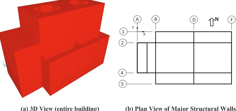
The selected structure, shown in Figure 1 (a) is a building representative of safety class nuclear facility structures with a footprint of 160 ft by 105 ft on a 6 ft mat foundation at El. 0 ft on the ground surface. The building is supported by reinforced concrete shear walls ranging in thickness from 2 ft to 3 ft. Four major shear walls provide lateral load resistance in the long (East-West (X)) direction of the structure (column lines 1, 2, 4, and 5) and four major shear walls provide resistance in the short (North-South (Y)) direction (column lines A, B, D, and F), as shown in the plan view in Figure 1 (b). The structure consists of 2 major floor slabs at El .33 ft and El. 62 ft, and a partial floor between column lines 2 and 4 at El 80 ft. All floors are reinforced concrete with thicknesses ranging from 2 ft to 3 ft. The roof is at El. 114 ft. The FE model of the structure is developed using shell elements for the mat foundation, walls and slabs.
Story drifts for the structure are calculated in the East-West (X) and North-South (Y) directions along a vertical line at the junction of major shear walls at the intersection of column lines 2 and B. The In-Structure Response Spectra (ISRS), considered for equipment fragility calculation, are also calculated at the same column line intersection at El. 33 ft slab.
(a) 3D View (entire building) (b) Plan View of Major Structural Walls
Figure 1. Case Study Structure
Limit state functions for drift ratios and ISRS at representative frequencies are considered for fragility calculation. In the case of drift ratios, failure is assumed at 0.5% inter-story drift with a log-SD of 0.335, where foundation rigid body rotation is excluded. For the considered structure, the 1st story drift (between El. 0 and 33 ft) in the Y direction and 2nd story drift (between El. 80.75 ft and 33 ft) in the X direction are most critical and considered in the fragility calculation.
The ISRS at the wall-slab joint (column lines 2 and B) on the 1st floor (El. 33 ft) are considered for the analysis. For the rock and soil site, different equipment with natural frequencies of 8 Hz, and 2 Hz, respectively, are selected. The equipment are assumed to have been designed using the 84th percentile
2 1
4
5
A B D N F
demand at the 1E-4 ground motion hazard level. The design demand for the equipment is assumed to correspond to 1 percentile on its capacity distribution curve, with a capacity log-SD of 0.3. The resulting design capacity and median capacity are 0.879 g and 1.77 g for the Rock case, and 0.450 g and 0.905 g for the Soil case.
Site Conditions
The following two sites are selected to represent two different sub-surface conditions:
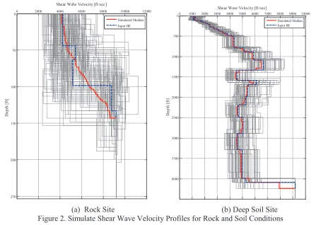
· A rock site with shear wave velocities starting at the ground surface level at around 4000 ft/sec and increasing gradually to around 5500 ft/sec in the upper 100 ft, followed by “hard rock”. Hard rock is characterized by a minimum shear wave velocity of 9200 ft/sec. The rock site is well investigated and its dynamic properties are well characterized (small epistemic uncertainty). However, the site measurements indicate a large aleatory variability, due to the highly variable and random nature of the rock weathering process, as demonstrated by a log-SD of 0.3 for the shear wave velocity in the top layers, see Figure 2 (a).
· A deep soil site where shear wave velocities in the upper 500 ft of soil increase gradually from about 1000 ft/sec to 4000 ft/sec. These layers are underlain by stiff layers of soil down to a depth of about 4000 ft where hard rock is found. The Soil site is not well investigated and only sparse data are available. The recommendations of the SPID report (EPRI, 2013) are adopted to characterize the aleatory variability, where a log-SD of 0.25 is assigned to the top 100 ft of soil and a log-SD of 0.15 is used for deeper soils, see Figure 2 (b). Same reference recommends the use of alternative soil columns to the Best Estimate (BE) to simulate the epistemic uncertainty about the adopted BE values. An epistemic log-SD of 0.35 is used to develop the two alternative soil columns, where the original BE profile is considered to be the 50th percentile with a weight of 40%, and the two alternative profiles are at the 10th and 90th percentiles, respectively, with weights of 30% each, refer to the SPID report for implementation details. The compounded uncertainty, accounting for both aleatory and epistemic contributions, amounts to an equivalent log-SD of 0.44 for the top 100 ft of soil.
Seismic Hazard
For the two selected sites, seismic hazard at the surface are available from the initial screening of the two sites following the recommendations of SPID report. The mean, median and fractile seismic hazard curves were calculated using approach 3 in NUREG/CR 6728 (McGuire et al., 2001). The log-SD as a function of ground motion intensity, Peak Ground Acceleration (PGA), are calculated by averaging the natural log of the ratio between the median (50th percentile) hazard curve and that of the 16th and 84th percentiles, respectively. The resulting hazard curves are presented in Figure 3 (a) and Figure 3 (b) for the rock and soil sites, respectively. Note that the calculated log-SD for seismic hazard curves accounts for both aleatory variability and epistemic uncertainty.
Parameter Uncertainty
23 Conference on Structural Mechanics in Reactor Technology Manchester, United Kingdom - August 10-14, 2015 Division VII
(a) Rock Site (b) Deep Soil Site Figure 2. Simulate Shear Wave Velocity Profiles for Rock and Soil Conditions
(a) Rock Site (b) Deep Soil Site Figure 3. Seismic Surface Hazard Curves for Rock and Soil Conditions
Table 1. Parameter Uncertainty
Engineering Parameter (Variable)
Best Estimate (BE)
Log-SD (ζ)
Total (epistemic and aleatory) Aleatory Variability
Ec 3,950 kip/in2 0.3 0.1
D 0.05 0.6 0.3
VS at surface (rock site) 4250 ft/sec 0.3 0.3
VS at surface (soil site) 870 ft/sec 0.44 0.25
0 2000 4000 6000 8000 10000 12000
0
50
100
150
200
250
Shear Wave Velocity [ft/sec]
D
e
p
th
[
ft
]
Simulated Median
Input BE
Simulated V
s Profiles (Top 253 ft)
0 1000 2000 3000 4000 5000 6000 7000 8000 9000 10000
0
500
1000
1500
2000
2500
3000
3500
4000
Shear Wave Velocity [ft/sec]
D
e
p
th
[
ft
]
Seismic Analysis
Probabilistic seismic site response analysis and probabilistic soil-structure interaction (P-SSI) analysis are performed to develop the median and statistical distribution of the considered seismic demands at 1E-4, 1E-5, and 1E-6 ground motion hazard levels. The entire probabilistic seismic analyses are carried out twice: once considering total composite uncertainties (estimates as the square root of sum of squares of the epistemic uncertainties and aleatory variabilities), and a second time considering only aleatory variability in the underlying parameters.
Probabilistic seismic site response analysis is carried out using PSHAKE (Deng and Ostadan, 2008) to develop the site specific surface hazard curves previously described (Figure 3) as well as the strain-compatible soil profiles corresponding to deaggregated (low frequency (LF) and high frequency (HF)) uniform hazard response spectra (UHRS) at the considered ground motion hazard levels.
P-SSI analysis is carried out in frequency domain using SASSI2010 (UC Berkeley, 2011), which employs random vibration theory in-lieu of using spectrum matched time-histories. For each ground motion hazard level (HF and LF at 1E-4, 1E-5, and 1E-6) and each of the 30 simulated LHS cases, a complete 3D SSI analysis of the example soil-structure system is carried out using ground motion input in X, Y, and Z directions. For the results from HF and LF events are enveloped to obtain the response at each of the 1E-4, 1E-5, and 1E-6 levels. While the horizontal motions are available through site response analysis and seismic hazard calculation, the vertical motions are calculated using appropriate V/H ratios.
The SSI analysis of the example structure is carried out to a cutoff frequency of 15 Hz for the soil site cases and 50 Hz for the rock site cases. Noting that the response of interest is composed of drift ratios, associated with low frequencies, and equipment demand accelerations at 2 Hz and 8 Hz, the cutoff frequency of the SSI analysis is considered adequate.
Fragility Function and Performance Calculation
The ISSFA fragility functions are calculated based on a three-point estimate. At each hazard level, and for each limit state function (LSF), the calculated demand parameters are approximated to a log-normal distribution. Noting that the capacity is also assumed to follow a log-normal distribution, the conditional failure probability at each hazard level is calculated using Equation 1:
ܲிȁீெ ൌ ͳ െ Ȱ ቆሺߣെ ߣሻ ටߞൗ ଶ ߞଶቇ (1)
where, Ȱ is the cumulative standard normal distribution function, ߣ, and ߣ are the logarithmic mean of the capacity and overall demand, respectively, and ߞ and ߞ are the logarithmic standard deviation of the capacity and overall demand, respectively. Using least-squares fit, a curve described by the exponential form ܨ௫Ψൌ ܨହΨή ሺȰିଵሺݔΨሻߚሻ is fitted to the three calculated probabilities of failure at three ground motion intensity levels, to estimate fragility curve median value (F50%) and corresponding uncertainty (β).
Performing this analysis for the set of realizations simulating aleatory variability allows for the calculation of βr, while the set of realizations simulating combined aleatory variability and epistemic uncertainty yields F50% and βc. The epistemic uncertainty contribution, βu is then calculated from ߚ௨ൌ
23 Conference on Structural Mechanics in Reactor Technology Manchester, United Kingdom - August 10-14, 2015 Division VII
Figure 4. Example Fragility Curves Considering Aleatory and Epistemic Components of Uncertainty
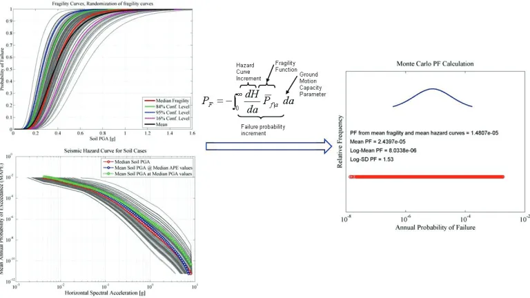
Using the median fragility function and its uncertainty, as well as the median hazard curve for PGA at surface and its uncertainty, a Monte Carlo (MC) simulation is carried out to convolve the two functions yielding the annual probability of failure and its uncertainty. The MC simulation is implemented using 1,000,000 realizations of the combinations of the fragility curves and hazard curves. As an example, Figure 5 provides the simulated fragility curves for the ISRS LSF (only the first 100 simulated curves are shown for clarity), simulated hazard curves (first 100 realizations), and the calculated annual probabilities of failure (PF) for the Soil site.
Figure 5. Calculation of the Annual Probability of Failure using Monte Carlo Simulation for ISRS LSF for Soil Case
selected structure is indeed very robust and unlikely to affect the overall seismic risk. However, as discussed earlier, we selected the capacities of the considered equipment using the site specific ISRS results, therefore their PF are more critical and are in the order of 3E-5.
An important observation is the large uncertainty estimated for the annual probability of failure (PF) for all LSF. In particular, for the ISRS LSF the logarithmic standard deviation (Log-SD) of PF is estimated as 0.98 and 1.53 for the rock and soil cases, respectively. Such large uncertainties suggest that 84th percentile of the PF is a factor of 2.7 for the rock case and 4.6 for the soil case higher than the median estimate. These high levels of uncertainty are representative of the values obtained in a typical SPRA and should be considered in discussion of SPRA results.
Table 2. Failure Probability, Fragility, and Performance Calculation for Drift Ratio LSF
Rock Site Soil Site
Composite Aleatory Composite Aleatory
PF | 1E-4 input 0 0 1.1E-08 3.6E-10
PF | 1E-5 input 3.0E-12 0 5.2E-05 1.4E-05
PF | 1E-6 input 8.6E-07 4.5E-09 2.7E-02 1.8E-02
Median Capacity [g] 21.5 1.02
βc 0.422 0.335
βr Not Calculated 0.313
βu Not Calculated 0.119
Mean PF (using mean curves) < 10-9 3.9E-07 Mean PF (using Monte Carlo) < 10-9 1.1E-06
Median PF < 10-9 1.9E-07
Log-SD of PF Not Calculated 1.84
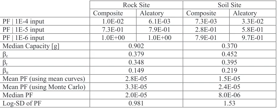
Table 3. Failure Probability, Fragility, and Performance Calculation for ISRS LSF
Rock Site Soil Site
Composite Aleatory Composite Aleatory PF | 1E-4 input 1.0E-02 6.1E-03 7.3E-03 3.3E-02 PF | 1E-5 input 7.3E-01 7.9E-01 2.8E-01 5.8E-01 PF | 1E-6 input 1.0E+00 1.0E+00 7.9E-01 9.7E-01
Median Capacity [g] 0.902 0.370
βc 0.379 0.452
βr 0.348 0.395
βu 0.149 0.219
Mean PF (using mean curves) 2.8E-05 1.5E-05 Mean PF (using Monte Carlo) 3.3E-05 2.4E-05
Median PF 2.0E-05 8.0E-06
Log-SD of PF 0.981 1.53
Sample Size Assessment
23rd Conference on Structural Mechanics in Reactor Technology Manchester, United Kingdom - August 10-14, 2015 Division VII
view of the large uncertainty characterizing the performance of the site-structure systems (log-SD greater than 0.8), therefore confirming the adequacy of the selected sample size.
Comparison with One-Point Estimate
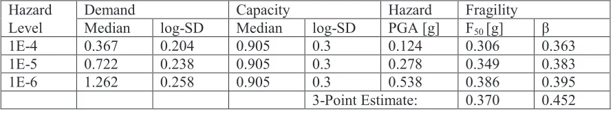
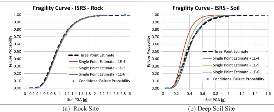
Fragility functions can be estimated by scaling of the review level earthquake (RLE, in most cases the 1E-4 hazard level) by the ratio of the capacity to demand in order to obtain the median ground motion capacity, thereby requiring the analysis of the site-structure system at one ground motion intensity level. This is a common practice in the nuclear industry today. The fragility function is constructed assuming exponential form, similar to three-point estimate, and with an added assumption that the log-SD for the failure probability at all hazard levels (more specifically at the RLE and at the median ground motion capacity) is the same. To evaluate the accuracy of this method, the one-point estimate fragilities and corresponding performances are calculated for the combined uncertainty cases. Table 4 and Table 5 present these results for the Rock and Soil sites, respectively, where one-point estimates are calculated for each of the three hazard levels (i.e. for the cases where RLE is assumed to be 1E-4, 1E-5, or 1E-6). The resulting fragility functions are plotted in Figure 6.
In the rock case, the one-point estimates for all three RLEs provide very close estimates of the F50 and β which are also very close to the three-point estimate results. This is due to the fact that the rock profile has little nonlinearity and the structure is assumed to be linear. In the soil case, which includes nonlinearity of the soil, the one-point estimates of the F50 for the three RLEs are different and range around the three-point estimate of the median capacity. On the other hand, the one-point estimates of the β value for the three RLEs underestimate the β value obtained from the three-point fragility method. The reason is that the uncertainty introduced by the scaling (i.e. assuming linearity between the RLE and median fragility point) in the one-point fragility estimation is neglected in this method. Although in general, this could lead to unconservative conclusions, the difference is relatively small and may be considered within the accuracy of most SPRA analyses. Nevertheless, the results indicate that where significant nonlinearity in the soil/structure system is expected, one-point estimates of the fragility curve should be viewed with caution.
Table 4. One-Point Estimate Fragility Functions for Rock Site
Hazard Demand Capacity Hazard Fragility Level Median log-SD Median log-SD PGA [g] F50 [g] β 1E-4 0.713 0.209 1.77 0.3 0.368 0.913 0.366 1E-5 2.232 0.210 1.77 0.3 1.181 0.937 0.366 1E-6 5.502 0.210 1.77 0.3 2.859 0.920 0.366 3-Point Estimate: 0.902 0.379
Table 5. One-Point Estimate Fragility Functions for Soil Site
(a) Rock Site (b) Deep Soil Site Figure 6. One-Point and Three-Point Fragility Function Comparison for ISRS LSF
Sensitivity of the Annual Probability of Failure and Its Log-SD to the Fragility and Hazard Uncertainties
The importance of different contributors to the estimation of the probability of failure (PF) and its uncertainty is investigated by setting the fragility curve epistemic uncertainty (βu), the fragility curve composite uncertainty (βc), or the uncertainty (log-SD) of the seismic hazard to zero, one-at-a-time (thus eliminating their effect) in the process of PF calculation. The results suggest that about 90% of the log-variance corresponding to the PF for the rock case and about 80% of the log-log-variance for the soil case are due to the uncertainty in the seismic hazard.
Also noted was that elimination of the fragility curve composite uncertainty (i.e. deterministic determination of failure) results in median PF estimates that are one to two orders of magnitude lower in both rock and soil cases than the rigorous cases considered. While this sensitivity study is not exhaustive, it nevertheless underlines the importance of accounting for the major sources of uncertainty in fragility and PF calculation, as accurately as possible.
CONCLUSIONS
· Very significant uncertainty exists in the calculated values for the annual probability of exceedance (PF, also known as the target performance goal). For the non-structural limit state functions (using ISRS) the mean PF is calculated as 3.3E-5 and 2.4E-5 for the rock and soil cases, respectively. The corresponding logarithmic standard deviations for these values are, respectively, 0.98 and 1.5. These results, while specific to the examples considered, are typical in their magnitude; similar levels of uncertainty in the calculated PF values should be expected across the industry.
· Seismic hazard uncertainty is the major contributor to the overall uncertainty in PF estimates, and should be taken into consideration. Careful consideration of the aleatory variability and epistemic uncertainty of the fragility curves allows development of fragility curve fractiles and more accurate median PF estimates, which in turn yield more consistent mean PF estimates. To reduce uncertainty in PF, the uncertainty in the seismic hazard needs to be reduced.
23rd Conference on Structural Mechanics in Reactor Technology Manchester, United Kingdom - August 10-14, 2015 Division VII
· In the rock case, which is mostly linear, the one-point fragility function estimates (fragility curve estimation using scaling from a single hazard level) for all three RLEs provide very close estimates of the F50 and β which are also very close to the three-point estimate results. This is due to the fact that the rock profile has little nonlinearity and the structure is assumed to be linear.
· In the soil case, which includes nonlinearity of the soil, the one-point estimates of the F50 for the three RLEs are different and they bound the three-point estimate of the median capacity. However, the one-point estimates of the β value for the three RLEs underestimate the β value obtained from the three-point fragility method. The reason is that the uncertainty introduced by the scaling inherent in the one-point fragility estimation is neglected in this method. In general, this could lead to unconservative conclusions, and suggests that where significant nonlinearity in the soil/structure system is expected, one-point estimates of the fragility curve should be viewed with caution.
REFERENCES
Deng N and Ostadan F "Random Vibration Theory Based Seismic Site Response Analysis," The 14th World Conference on Earthquake Engineering, October 12-17, 2008, Beijing, China, Paper 04-02-0024.
Electric Power Research Institute (EPRI) “Seismic Evaluation Guidance: Screening, Prioritization and Implementation Details (SPID) for the Resolution of Fukushima Near-Term Task Force Recommendation 2.1: Seismic,” EPRI Final Report, Report 1025287, February 2013.
Elkhoraibi TE and Hashemi A “Integrated Soil-Structure Fragility Analysis Method for Nuclear Structures,” Fifth International Conference on Earthquake Geotechnical Engineering. Santiago, Chile, 10–13 January 2011.
Elkhoraibi T, Hashemi A, and Farhang O “Probabilistic and Deterministic Soil Structure Interaction Analysis Including Ground Motion Incoherency Effects,” Nuclear Engineering and Design, V. 269, 1 April, 2014.
Hashemi A, Elkhoraibi T, and Ostadan F “Probabilistic and Deterministic Soil Structure Interaction (SSI) Analysis.” Eleventh International Conference on Application of Statistics and Probability in Civil Engineering (ICASP11), ETH Zurich, Switzerland, 1–4 August 2011.
Hashemi A, Malushte S, Saini J, and Moreschi L “Improved Tow-Step Method for Seismic Analysis of Structures,” Tenth U.S. National Conference on Earthquake Engineering (10NCEE), Anchorage, Alaska, USA, July 21-25, 2014.
Hashemi A, Elkhoraibi T, and Farhang O “Effects of Structural Nonlinearity and Foundation Sliding on Probabilistic Response of a Nuclear Structure,” Nuclear Engineering and Design, In Press, 2015. McGuire RK, Silva WJ and Costantino CJ “Technical Basis for Revision of Regulatory Guidance on
Design Ground Motions: Hazard- and Risk-Consistent Ground Motion Spectra Guidelines”, NUREG/CR-6728, U.S. Nuclear Regulatory Commission, Washington, D.C., 2001.
McKay MD, Beckman RJ and Conover WJ “A Comparison of Three Methods for Selecting Values of Input Variables in the Analysis of Output from a Computer Code” Technometrics, Vol. 21, Issue 2, pp. 239-245, 1979.