NALWAYA, AKSHAY. Using Hoeffding Sampling and Project Elimination to make Bellwether Discovery Faster. (Under the direction of Dr. Timothy Menzies).
In software engineering, the project data is continuously updated and augmented.
Prediction models build from these projects become increasingly varied as the number of projects
increased and ultimately resulting in changing results. This problem of conclusion instability in
software engineering can be mitigated by using Bellwethers. It helps to build quality software
prediction models. This problem was extensively researched in paper Bellwethers. Bellwethers are
used as a baseline method for transfer learning and then this baseline is used for comparing future
models.
So, in this work, we explore alternative methods to make the task of identification of
bellwethers project in a group of projects faster for the defect prediction domain. An O(N2)
approach was presented in the Bellwethers paper and we try to explore the applicability of
Hoeffdings bounds to sample the training set and experiment with various combinations in the
train and test sets. In addition to sampling the dataset, we also try to prune projects which are
unlikely to be a candidate for the bellwether project. Then we perform experiments with various
feature selection algorithms with the aim to reduce the bellwether identification time and improve
© Copyright 2019 by Akshay Nalwaya
by
Akshay Nalwaya
A thesis submitted to the Graduate Faculty of North Carolina State University
in partial fulfillment of the requirements for the Degree of
Master of Science
Computer Science
Raleigh, North Carolina
2019
APPROVED BY:
______________________________ _______________________________ Dr. Timothy Menzies Dr. Matthias Stallmann
Committee Chair
ii
BIOGRAPHY
Akshay Nalwaya was born in a small town named Ratlam in India. He obtained his
bachelor’s degree in Computer Engineering from Shri GS Institute of Technology and Science in
2016. After that, he joined Mu Sigma as a Decision Scientist. In 2017, Akshay started his master’s
degree in Computer Science at NC State University and joined ABB as an Artificial Intelligence
Intern after a year. To explore research in the areas of machine learning and data science, Akshay
iii
ACKNOWLEDGMENTS
I would like to thank Professor Timothy Menzies for giving me an opportunity to work
and explore Bellwethers phenomenon in software engineering projects and providing an
introduction about various concepts of data mining for Software Engineering in general. I would
also like to express my gratitude towards Rahul Krishna for helping at various times of need and
iv
TABLE OF CONTENTS
LIST OF TABLES ... v
LIST OF FIGURES ... vi
Chapter 1: Introduction ... 1
Bellwethers ... 1
Importance of bellwether identification ... 1
Defect Prediction ... 2
Research Questions ... 3
Statement of Thesis ... 4
Contributions... 4
Structure of Thesis ... 5
Chapter 2: Related Work ... 6
Chapter 3: Core Idea ... 8
Proposed Solution ... 8
Hoeffding Bounds ... 9
Sampling using Hoeffding Bounds ... 10
Modifying Hoeffding Bounds to reduce time ... 11
Project Elimination ... 12
Feature Selection ... 14
Importance of Feature Selection ... 15
Forward Feature Selection ... 16
Backward Feature Elimination ... 17
Information Gain as a feature selector ... 17
Correlation-based feature selection ... 19
Chapter 4: Experimental Design ... 20
Dataset... 20
Baseline Model ... 21
Model Evaluation ... 21
Standard Measures of Evaluation ... 22
Class Imbalance ... 23
Chapter 5: Results... 25
RQ1: Can we predict which data set is Bellwether? ... 25
RQ2: Can we reduce the time to find bellwether by reducing the size of data? ... 26
RQ3: Does sampling data using Hoeffding bounds outperform project elimination? ... 28
RQ4: Does feature selection improve the performance of bellwether identification? ... 28
Chapter 6: Conclusion ... 30
Conclusion ... 30
Future Work ... 31
v
LIST OF TABLES
Table 4.1 Data points for each project in Jureczko ... 20
Table 5.1 Median G-Score values for different approaches for Bellwether prediction ... 25
Table 5.2 Comparing run-times of all approaches for Bellwether identification ... 27
Table 5.3 Percentage of data required for training on a project and testing on others using Hoeffding bounds ... 28
Table 5.4 Projects pruned during project elimination approach ... 28
Table 5.5 G-Scores from project elimination approach ... 28
Table 5.6 Comparison of various feature selection algorithms for ‘poi’ ... 29
vi
LIST OF FIGURES
Figure 3.1 High-level process flow of proposed approach for Bellwether identification ... 9
Figure 5.1 Median g-score for ‘poi’ was the highest among all projects ... 26
Figure 5.2 Average runtime values for Bellwether identification ... 27
1
CHAPTER 1: INTRODUCTION Bellwethers
The bellwether effect described in Bellwethers[1] states that when a community works on
software, then there exists one exemplary project, called the bellwether, which can make
predictions for the others. The model built using a bellwether project can serve as a baseline model
for constructing different transfer learners in various domains of software engineering.
Bellwethers use the concept of transfer learning. When there is insufficient data to apply
data miners to learn defect predictors, transfer learning can be used to transfer lessons learned from
other source projects to new projects. Suppose, there is a new project, so we wouldn't have enough
data for it, to predict the defects. This is when we can use data from other projects to make
predictions for new projects.
Importance of bellwether identification
If there is insufficient data, transfer learning can be used by data miners and they could use
lessons learned from one project and apply them on another project. Since the probability of having
a defective code and a non-defective code is not similar, the SE data is often imbalanced and
difficult to get. In such cases, Bellwethers method presents a simple solution - instead of exploring
all available data, find one data set that may offer a stable conclusion over a longer period.
Bellwethers[1] shows the existence of such projects in SE data sets and strives to find them. It is
true that bellwethers, with such simplicity, are always better than other complex algorithms used
for similar applications. At the same time, it has been shown that bellwethers are capable of
2
Defect Prediction
The programs written for software engineering have various flaws. Every piece of code
should be tested before addition to the main repository. The software can crash or malfunction if
the code has defects. These parts of code that can lead to malfunction or even crash of
application are called defects. Now, a possible solution to avoid defects is by testing the code
beforehand. However, testing introduces a lot of additional expenses and sometimes the time
taken for testing is similar to the time taken for developing that piece of code. This regards
testing as a possible solution but not an optimum solution. Tim Menzies in his paper [2] correctly
mentions that, the fundamental issue in cross project defect prediction is selecting the most
appropriate training data for creating quality defect predictors. Another concern is whether
historical data of open-source projects can be used to create quality predictors for proprietary
projects from a practical point-of-view. Also these methods apply brute force techniques which
are computationally expensive. Exponential costs exhaust the resources available and testing
could be made less expensive, if only a part i.e., a critical section has to be tested.
There are various approaches to find such critical section in the code. For example, the
defect predictions can be made using static code attributes. So, once the miner learns which
section of code is most likely to have a defect, it can make predictions. Another method,
although more time consuming is manually going through the code, which is more accurate. So,
these methods can be used to guide which sections of code might have defects. The defect
prediction models prioritize code review as well as testing resources, hence making them easier
to use. Additionally, defect predictors often find the location of 70% (or more) of the defects in
3
Research Questions
• RQ1: Can we predict which data set is bellwether?
For identifying a Bellwether we take the Jureczko repository for defect predictions, we
built a Random Forest Classifier using the approach mentioned in the Bellwethers[1] paper and
compare these results with different sampling and elimination techniques as discussed in the
subsequent sections. Based on the results obtained, we were able to find the Bellwether project
and it was the same in all the different implementations. This also shows that there exists a project
which can act as a predictor for all the other projects.
• RQ2: Can we reduce the time to find bellwether by reducing the size of data?
We tried different algorithms that explore the possibility of not requiring to test current
project against every other project or to reduce the data instances required for training/testing. For
this, we have applied Hoeffding bounds and project elimination. It was found that Hoeffding
bounds reduced the bellwether identification time significantly by reducing the amount of training
data needed. Then project elimination was implemented which also reduced the runtime by a
fraction of N.
• RQ3: Does sampling data based on Hoeffding sampling outperforms idea of project
elimination?
We studied the results obtained by the baseline model and established a threshold value for
G-score that each project should satisfy to be considered for being a bellwether. This cut-off helped
to eliminated certain projects that performed poorly for other projects. The time is taken by this
4 were almost similar to those obtained by baseline and sampling techniques showing that without
any loss in identification accuracy, we are able to reduce the run-time significantly.
• RQ4: Does feature selection improve the performance of the bellwether identification?
We implemented feature selection using algorithms that select a subset of features using
information gain, and correlation. Also, we implemented forward and backward feature selection
and performed a comparative study of their effect on bellwether prediction. It was found that the
additional time taken by these approaches was not proportional to the improvement in g-score.
Statement of Thesis
Based on the experiments, it can be concluded that the current approach for finding
bellwethers has high time complexity and can be reduced by using sampling techniques and project
elimination.
Contributions
This work shows that by incorporating these concepts into bellwether identification
approach the time complexity can be reduced without any compromise on the performance of the
model. A new heuristic for project elimination has been proposed and implemented which takes
use of the domain knowledge of the projects and determines the elimination threshold for
eliminating projects. Feature selection is also incorporated to study the effect of various feature
5
Structure of Thesis
The rest of the thesis is organized as follows. Chapter 2 describes the work already done in
this field and the merits/demerits of those approaches. Chapter 3 explains the core idea behind this
thesis, the motivation behind it, followed by the algorithm proposed. Chapter 4 lays out the
experimental design and the experimental trials performed. Chapter 5 presents the result of the
experiments with respect to each of the research questions discussed above. Chapter 6 explains the
6
CHAPTER 2: RELATED WORK
The current methodology of bellwether identification is an O(N2) algorithm that tends to evaluate each project against every other project. Though this is a simple process we believe that
this approach needs investigation. In the current solution, data sets from a community are taken.
Suppose we have 10 data sets, each data set is used for training a model. A model trained on a data
set is tested on the remaining 9 data set. Relevant evaluation metric values are found. The model
that makes the best predictions for most of the data set is found. The data set that was used to train
this model is identified as Bellwethers. Evaluation metric generally used is G-score.
Identifying a bellwether project and using it for making predictions for the rest of the
projects in that domain is a novel concept. This eliminates the need for training a model for each
of the project for defect prediction. The time consumed for this approach would be very high as
the number of projects keep on increasing. So, another approach that reduces the time complexity
should be researched in order to make this algorithm applicable even when the number of projects
increase.
It is important that the solution is scalable owning to the exponentially increasing data.
This is issue is brought up by Zhang et. al. in their paper [3]. They mentioned, "Due to the large
scale of the data being analyzed, analytic technologies such as machine learning techniques need
to be scalable. The realization of scalability includes both the design and implementation of
analytic technologies."
Predicting defective parts of the software that are more likely to contain defects. This effort
is particularly useful when the project budget is limited, or the whole software system is too large
to be tested exhaustively. A good defect predictor can guide software engineers to focus the testing
7 Bellwethers. Once we have the bellwethers data set, we can use it to predict defects for other
projects. This will be extremely helpful not only when we there is no relevant amount of data for
the new project but also, using just one data set and trained model we can predict defects for
various projects.
For a high-performance defect predictor, researchers have been working on the choice of
static attributes and effective learning algorithms since the 1990s [5]. The McCabe [6] and
Halstead [7] metrics are widely used to describe the attributes of each software module (i.e. the
unit of functionality of source code). In addition to seeking a better subset of attributes, choosing
a good learning algorithm was shown to be at least equally important to the final performance [8].
Various statistical and machine learning methods have been investigated for SDP (Software Defect
Prediction), among which Naive Bayes [8] and Random Forest [9], [10] were shown to have
relatively high, stable performance [9], [11]. AdaBoost based on C4.5 decision trees was also
found to be effective in some studies [12], [13].
Although bellwether identification used above is a simple process, we believe that this
approach needs investigation. We can clearly see that the issue of runtime complexity remains an
open issue and hence this thesis is to present another approach that can perform the same task with
8
CHAPTER 3: CORE IDEA Proposed Solution
As mentioned in the previous chapter, the current methodology of bellwether identification
is an O(N2) algorithm that tends to evaluate each project against every other project. We aim to find a method that identifies a bellwether project in much lesser time without introducing any
unnecessary complexity in the identification process. Also, it should be scalable when the number
of projects is much larger than the ones explored in the current approach.
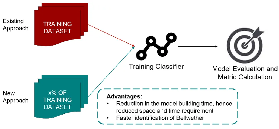
We can sample each data set to reduce the training or testing data set. This should lead to
a significant reduction in the data set size, hence, reducing the time required to find the bellwethers.
We performed various experiments with sampling the training and testing data sets. In addition to
just sampling the data sets, we also compare this sampling method with the idea of eliminating a
project altogether without having to test it on all the projects. For this we explored sampling
methods available and zeroed on Hoeffdings bound method. This sampled the project data only
till an improvement in the results can be obtained, this ensures that only required data points are
chosen for training. This decreased the unimportant data points and hence lesser redundancy.
Sampling the training data would still require performing the training and testing on the
sampled data set for each of the combination of projects in the repository. If we can eliminate some
projects with low performance based on their performance in the initial stages, then it would give
a much faster bellwether identification. This will reduce the number of projects that the algorithm
will have to train the model on and hence would keep on shrinking the pool of candidate bellwether
9
Figure 3.1 High-level process flow of proposed approach for Bellwether identification
Hoeffding Bounds
Let us say that we have N points with which to test a given model. If we were to test a
model on all of them, then we would have an average error that we will call Etrue. However, if we
only tested the model on ten points, then we only have an estimate of the true average error. We
call the average after only n points (n<N)Eest since it is an estimate of Etrue. The more points we
test on (the bigger n gets), the closer our estimate gets to the true error. How close is Eest to Etrue
after n points? Hoeffding bound lets us answer that question when the n points are picked with an
identical independent distribution from the set of N original test points. In this case, we can say
that the probability of Eest being more than away from Etrue
Pr(|𝐸𝑡𝑟𝑢𝑒− 𝐸𝑒𝑠𝑡| > 𝜖) < 2𝑒−2𝑛𝜖2⁄𝐵2
where B bounds the greatest possible error that a model can make [16]. This bound does
not make any assumptions other than the independence of the samples. The hoeffding racing
10 Hoeffding racing algorithm has three major steps. It starts with each model known as the
learning box. Learning box can be complex or time-consuming, we consider just the input and
output of the model. The error is one of the most important metrics. Testing set is taken one data
point at a time and data points are added. At each addition of data point, the error is calculated. So,
firstly, compute the leave-one-out cross-validation error at each point of the test data set. The
average error rate is updated at each iteration, as data points are added to the test data set. Using
Hoeffding bound, we calculate how close is the average error rate to the original error rate. We
can eliminate those learning boxes whose best possible error is still greater than the worst error of
the best learning box. The point at which hoeffding bound is hit, we can break the loop. Racing
algorithms basically, learn from the good models and eliminate the bad ones.\newline
Since racing never performs more queries than brute force, we formulated a strategy to use
this in order to find Bellwethers. Also, the overhead involved in this process is negligible.
Sampling using Hoeffding Bounds
In this approach, our motive was to decrease the time required to find Bellwethers by
decreasing the training data set. Each data set was taken, and the samples were added to the training
data set. We start with 5% of the data set and at each iteration, 1% of the data is added. Model is
trained on this data at each iteration and tested on the other projects. The point at which we are
95% confident that our estimate of the running g score is within the epsilon of baseline g-score is
noted. The loop breaks for that test project and runs for all the remaining test projects. Once, we
hit hoeffding bound for each test project, a similar exercise is run for the remaining projects. This
11 However, the fraction of data being sampled for each test project was different. Hence, the
time taken to run the process was not reduced. The fact that sampling the training data set for each
test set was increasing the time of execution led us to devise another approach.
Algorithm
start time = current time for project in projects read data
for testproj in projects
if testproj not equal to project
sample data upto hoeffding bound train random forest classifier make predictions on testproj calculate gscore
append g to a table end time = current time
runtime = end time - start time
Modifying Hoeffding bounds to reduce time
In order to eliminate the time taken for sampling the training data differently for each data
set, we took the maximum of the percentage of data required by any test project. This did not just
decrease the training data set but impacted the time taken to find bellwethers. The time taken to
find Bellwethers was reduced by 4 times.
In this approach, the sampling of data was done just once, and with the reduced training
data set, predictions are made following the similar steps:
Firstly, each data set was taken, and the samples were added to the training data set. We
start with 5% of the data set and at each iteration, 1% of the data is added. Model is trained on this
data at each iteration and tested on the other projects. The point at which we are 95% confident
that our estimate of the running g-score is within the epsilon of baseline g-score is noted. The loop
breaks for that test project and runs for all the remaining test projects. Once, we hit hoeffding
12 project, we consider the maximum amount of data required by any other test project. The training
data is sampled according to the results from previous steps.
Bellwether prediction is done using the g-scores calculated according to the predictions
made for each test data set. This helped us reduce the training data considerably as well as reduce
the time by 4 times. G-scores calculated is almost similar to the values calculated through the
baseline method.
Algorithm
start time = current time for project in projects read data
frac = get max % of training data sample data for frac
train random forest classifier for testproj in projects
if testproj not equal to project make predictions on testproj calculate gscore
append g to a table end time = current time
runtime = end time - start time
Project Elimination
In the above experiments, we focused on using Hoeffding Bounds for efficiently sampling
the data sets for all the projects. Depending on the approach, we experimented with sampling only
the training data, or testing data, and then sampling both: training and testing data. The end goal
was to try and reduce the number of records to be used for training and testing purposes. This
doesn't reduce the number of projects, but it reduces the constant term in run-time complexity
analysis, i.e., in N2 the term c is reduced.
In this experiment, our objective was to explore if we can eliminate some projects and
13 for all the projects and found that some projects which consistently had low values for G-score for
a prediction on other projects continued this trend for all the projects. This accounted for a large
amount of time being spent on training and testing of projects that were not the candidates for
bellwether. So, such projects should be eliminated without spending time using such projects for
testing for all other projects.
Based on the baseline G-score values we decided a threshold value for the G-score. This
threshold value should be satisfied for all the projects in order to be considered as a candidate
bellwether project. The central value of G-score distribution for all the projects was chosen as the
threshold value. Mean, median and mode are the most commonly used measures of central
tendency. We chose the median as the representative value of the central tendency for bellwethers
since mean is prone to be influenced by the presence of outliers in the data (G-score of projects in
this case). One project with very low G-score could bring down the threshold G-score and lead to
increased processing time. On the other hand, the median is not affected by some outliers in data,
and hence is a better measure for this case.
Once this threshold was decided, we started with training a Random Forest Classifier on
each of the projects. This trained random forest classifier is used for testing on all the other projects
in a sequential manner. The G-score values for each iteration are recorded for each of the trained
classifier models. The current project is eliminated if the following two conditions are satisfied:
1. Condition 1: Project is tested on at least 1/3rd of the projects
2. Condition 2: Mean of G-score value is less than the specified threshold value
All the projects satisfying these conditions are tested for the other projects until they violate
these conditions, or it has been tested on all available projects. The projects violating these
14 the early stopping rule to avoid testing on all projects and efficiently reducing the number of
projects used for testing.
The G-score values are then aggregated for projects that have not been eliminated. The
median value of G-score is taken and reported as the G-score for each project and the project with
the highest mean value of G-score for testing on other projects is termed as the bellwether project
for the given set of projects.
Algorithm
for each project do
load X_train, y_train
train random forest classifier set threshold g-score
for all other projects load X_test, y_test make predictions compute g-score
if eliminate-count > 2: break
if g-score < threshold && #projects tested >= 3: g-score = 0
append results, g-score
return results
Feature Selection
Although the above approaches reduce the time taken for Bellwether identification, we can
try to reduce the time further by using feature selection techniques. Currently, we use the random
forest classifier for building the classification model and it generates an ensemble of decision trees
during the training phase. The final prediction by the model is based on the collective predictions
from all these trees generated during the intermediate phase. This avoids overfitting in this
15 Feature selection can be defined as the process of choosing a minimum subset of M features
from the original set of N features so that the feature space is optimally reduced according to
certain evaluation criterion. Feature selection reduces the dimensionality of feature space, removes
redundant, irrelevant, or noisy data. It brings the immediate effects for application: speeding up a
data mining algorithm, improving the data quality and thereof the performance of data mining, and
increasing the comprehensibility of the mining results. [18]
We thought of using feature selection techniques into the approach with the objective of
improving the performance of the system and reducing the time taken for the identification of
bellwether project. Since only a subset of features will be present in the training data, the runtime
for training the model should decrease.
Importance of Feature Selection
The main idea behind feature selection is to keep the relevant features in the data while
removing the irrelevant features. This is done because the irrelevant attributes can degrade the
performance of the model and they give no information about the final class variable to be
predicted. Some of the key advantages of using feature selection are:
• Reduction in overfitting since predictions would now be made based on important
features
• Improves the performance of the model
• Since training data reduces, training time decreases
Because of all these advantages offered by feature selection, we chose a few feature
selection algorithms and analyzed their effect on the overall time and performance of the system.
• Forward Feature Selection
16 • Information Gain as a feature selector
• Correlation-based feature selection (CFS)
Forward Feature Selection
This is a feature selection approach where features are added to the selected subset of
features one-by-one in each iteration until the addition of that features gives an improvement in
the model. This process is iterative and it begins with an empty set in which we start with one of
the features from the set of all features available in the data. Next step is to train a classifier model
and measure its performance. The model evaluation metric, g-score in this case, is calculated. Now,
another feature is selected from the set of features and added to this subset. The same process is
repeated and the new g-score is compared with the previous g-score. The process stops when the
new g-score value is lower than the previous g-score value indicating that the model performance
has started degrading and the current subset of features is selected.
Algorithm:
create empty feature_subset
while (feature_subset does not contain all features):
add another feature to feature_subset
train random forest classifier on feature_subset
make predictions
calculate the g_score and store as new_gscore
if new_score < old_score:
break
old_score = new_score
17
Backward Feature Elimination
This feature selection approach works in the opposite way as compared to the forward
feature selection approach. In this approach, we start with a set containing all the features from
data and keep on iteratively removing the features until the performance of the model improves.
The terminating condition of this iterative process is the same as the forward selection approach.
The rationale for this approach was that forward selection might stop early if the performance
degrades but some important features might not have been used till now. This is because of the
sequential manner of operation of these approaches.
Algorithm:
create feature_subset having all the features
while (feature_subset is not empty):
remove a feature from feature_subset
train random forest classifier on feature_subset
make predictions
calculate the g_score and store as new_gscore
if new_score < old_score:
break
old_score = new_score
return feature_subset
Information Gain as a feature selector
Both forward selection and backward elimination algorithms proceed in a sequential
manner and hence, might terminate while encountering one or few of the irrelevant features. This
will result in a suboptimal subset of features being selected by the algorithm. But, if we use
information gain as a metric for feature selection [2], it ensures that features are selected in order
18 It is one of the fastest methods for feature selection because we are not required to train the
classifier model at each iteration, rather we compute the information gain for all attributes and then
make a selection of feature subset. Once this feature subset is selected, the classifier model is
trained on the data.
Entropy and Information Gain: Entropy of an attribute is the measure of its degree of randomness in a set of data points. The amount by which the entropy of the class decreases reflects
the additional information about the class provided by the attribute and is referred to as the
information gain. [2] Mathematically,
𝐻(𝐶) = − ∑ 𝑝(𝑐) log2𝑝(𝑐) 𝑐 ∈ 𝐶
𝐻(𝐶|𝐴) = − ∑ 𝑝(𝑎)
𝑎 ∈ 𝐴
∑ 𝑝(𝑐|𝑎) log2𝑝(𝑐|𝑎) 𝑐 ∈ 𝐶
where, H(C) represents the entropy of class C,
H(C|A) represents the entropy of class C given attribute A.
Information gain for each attribute is calculated using,
𝐼𝐺𝑖 = 𝐻(𝐶) − 𝐻(𝐶|𝐴𝑖)
= 𝐻(𝐴𝑖) − 𝐻(𝐴𝑖|𝐶)
= 𝐻(𝐴𝑖) + 𝐻(𝐶) − 𝐻(𝐴𝑖, 𝐶)
where, IGi represents the information gain for attribute Ai.
Algorithm:
Calculate info. gain for all attributes w.r.t. class
variable
importance = list of information gain values
19
for all features:
if info. gain > threshold:
add it to feature_subset
return feature_subset
Correlation-based feature selection (CFS)
The main approach that differentiates CFS from all the algorithms discussed above is that
it evaluates a subset of attributes rather than evaluating each attribute individually. This ensures
the consideration of the level of inter-correlation between attributes while choosing the optimal
subset during feature selection. A score is assigned to each candidate subset of attributes which is
called merit. For a subset S, the value of merit is calculated as,
where, k is the number of features,
𝑟̅̅̅̅𝑐𝑓 is the average feature-class correlation,
𝑟̅̅̅̅𝑓𝑓 is the average feature-feature inter-correlation,
Based on this heuristic, CFS would assign high scores to subsets with attributes having a
20
CHAPTER 4: EXPERIMENTAL DESIGN Dataset
We limited our work to finding Bellwethers for defect measures we relied on data set
gathered by Jureczko [17]. The data set contains defect measures from several Apache projects.
The data set comprises data from 10 different projects. This data set contains records the number
of known defects for each class using a post-release bug tracking system. The classes are described
in terms of 20 metrics. Each data set in the Apache community has several versions. We merged
data set across different version to create a bigger data set.
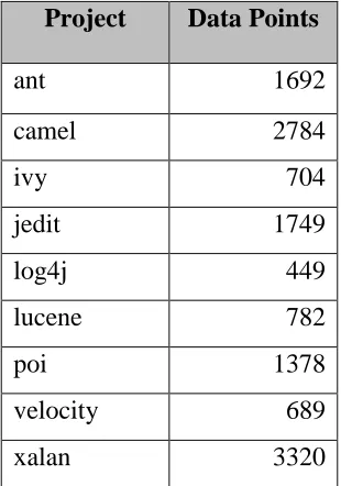
Following are the details of the data set for each project. All projects had 20 features. Since
the class variable was continuous, we performed pre-processing to convert it to binary. This was
done because our objective was to find whether for a given instance, will it have a bug or not and
not the number of bugs identified. So, we mapped all the instances having at least 1 bug as a
positive class (1) while those not having any bug as the negative class (0).
Table 4.1 Data points for each project in Jureczko
Project Data Points
ant 1692
camel 2784
ivy 704
jedit 1749
log4j 449
lucene 782
poi 1378
velocity 689
21
Baseline Model
There are many binary classifiers to predict defects, the Bellwethers [1] cites studies on
defect prediction and follows the use of Random Forests for defect prediction over several other
methods. For the sake of simplicity and effective comparison (if required) we decided to use the
Random Forest Classifier.
Baseline calculation is a straight forward task - for each project in the community train the
model and test it against every other project and compute g-scores for each of the test iterations.
The project with the best median value of the g-score is declared the Bellwether.
Algorithm
start time = current time
for project in projects
read data
train random forest classifier
for testproj in projects
if testproj not equal to project
make predictions on testproj
calculate gscore
append g to a table
end time = current time
runtime = end time - start time
Model Evaluation
The data set under consideration has binary class labels, with the records belonging to
either the positive or negative class. The instances of projects having defects (one or more) are
assigned a positive class while those without defects are assigned negative class implying no defect
22 There are various metrics that can be derived from the confusion matrix obtained as a result
of testing the classifier on each of the projects. Different measures of model evaluation are
summarized below:
Standard Measures of Evaluation
• Accuracy – It is the percentage of instances of the data set that have been classified
correctly by the model. It emphasizes on correct classification of both positive and
negative classes equally. The mathematical formula for accuracy is,
𝑎𝑐𝑐𝑢𝑟𝑎𝑐𝑦 = 𝑡𝑟𝑢𝑒 𝑝𝑜𝑠𝑖𝑡𝑖𝑣𝑒 + 𝑡𝑟𝑢𝑒 𝑛𝑒𝑔𝑎𝑡𝑖𝑣𝑒 𝑡𝑜𝑡𝑎𝑙 𝑛𝑢𝑚𝑏𝑒𝑟 𝑜𝑓 𝑖𝑛𝑠𝑡𝑎𝑛𝑐𝑒𝑠
• Precision – It talks about how precise your model is, meaning it shows what fraction
of instances that are predicted positive, are actually positive. Hence, a model with low
precision would imply that either a there was a large number of false positives in the
model or the number of true positives was very low.
𝑃𝑟𝑒𝑐𝑖𝑠𝑖𝑜𝑛 = 𝑡𝑟𝑢𝑒 𝑝𝑜𝑠𝑖𝑡𝑖𝑣𝑒
𝑡𝑟𝑢𝑒 𝑝𝑜𝑠𝑖𝑡𝑖𝑣𝑒 + 𝑓𝑎𝑙𝑠𝑒 𝑝𝑜𝑠𝑖𝑡𝑖𝑣𝑒
• Recall – It calculates how many of the actual positive instances have been correctly
captured by the model (true positives). It is also denoted by pd or the probability of
detection.
𝑅𝑒𝑐𝑎𝑙𝑙 = 𝑡𝑟𝑢𝑒 𝑝𝑜𝑠𝑖𝑡𝑖𝑣𝑒
𝑡𝑟𝑢𝑒 𝑝𝑜𝑠𝑖𝑡𝑖𝑣𝑒 + 𝑓𝑎𝑙𝑠𝑒 𝑛𝑒𝑔𝑎𝑡𝑖𝑣𝑒
• False Alarm – As the name suggests, this metric gives the percentage of negative
instances that were erroneously predicted as positive instances. It is also denoted by pf.
𝑝𝑓 = 𝑓𝑎𝑙𝑠𝑒 𝑝𝑜𝑠𝑖𝑡𝑖𝑣𝑒
23 Each of the metrics we discussed above is used for model evaluation depending on the
application and the type of data. For instance, if one aims to increase the recall for a model, then
it might also increase the false alarm (pf) of the model. Similarly, there is a kind of inverse
relationship present in between precision and recall. If one tries to increase the precision of a
model, then the recall might have to be compromised with.
Class Imbalance
Class Imbalance in classification problems is a scenario where classes are not represented
equally. Most classification data sets do not have an equal representation of the classes and often
such class imbalance needs careful handling. Slight variations in the class distributions can be
ignored but a significant variation needs to be taken into account.
There are several ways of handling class imbalance and most common among them are:
• Collect more data
• Change performance metric
• Re-sampling data set
Why not choose accuracy for model evaluation in case of data with class imbalance?
In the cases discussed above, accuracy can often be misleading. At times it may be
desirable to select a model with a lower accuracy because of better predictive power on the
problem. This issue is also explained Sokolova et. al. in their paper [4]. They mention, "the most
used empirical measure, accuracy, does not distinguish between the number of correct labels of
different classes."
For example, in a problem where there is a large class imbalance, a model can just predict
the value of the majority class for all predictions and achieve a high classification accuracy, the
24
Model evaluation metric for class imbalance : G-Score
We use the g-score [14] [15] as a metric for evaluating performance of classifier in this
case of class imbalance. It combines recall (pd) and false alarm rate (pf). The Bellwethers [1] cites
studies which suggest that such a measure is justifiably better than other measures when the data
set has imbalanced distribution in terms of classes. Hence, we are using G-Score in this paper as
well. G-Score is measured as follows:
𝐺 =2 ∗ 𝑝𝑑 ∗ (1 − 𝑝𝑓) (1 + 𝑝𝑑 − 𝑝𝑓)
For example, in a problem where there is a large class imbalance, a model can just predict
the value of the majority class for all predictions and achieve a high classification accuracy, the
25
CHAPTER 5: RESULTS
RQ1: Can we predict which data set is Bellwether?
We can predict bellwethers using the baseline method, and this method generates g-score
values. It should be noted that the value of g-score for all the approaches discussed in this paper is
very similar.
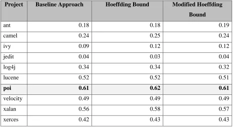
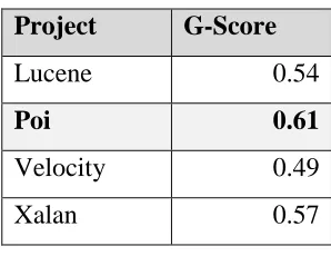
The bellwether data set can be predicted using the g-score and poi, proves to be the data
set with the best g-score. However, xalan and lucene have median g-score comparable to that of
poi. We implemented three different approaches to predict Bellwethers and for all the three
approaches, poi has the highest g-score throughout.
Table 5.1 Median G-Score values for different approaches for Bellwether prediction
Project Baseline Approach Hoeffding Bound Modified Hoeffding Bound
ant 0.18 0.18 0.19
camel 0.24 0.25 0.24
ivy 0.09 0.12 0.12
jedit 0.04 0.03 0.04
log4j 0.34 0.34 0.32
lucene 0.52 0.52 0.51
poi 0.61 0.62 0.61
velocity 0.49 0.49 0.49
xalan 0.56 0.58 0.57
26
RQ2: Can we reduce the time to find bellwether by reducing the size of data?
For research question 2, we found the point when hoeffding bound is hit. Instead of the
whole training data set, only a percentage of the data set sample can be taken. The results are
shown in the table below. All results were calculated after running for 30 iterations.
The data for training can be reduced a lot but sampling the data, again and again, consumes
a lot of time. Hence, we took the maximum amount of training data required to hit the hoeffding
bound for any test project and sampled training data accordingly. The sampling of data for each
training set is just done once, considerably reducing run time. The results show that the run time
has reduced more than 4 times. Tables below show the percentage of data used for training, their
updated G-score and the runtimes for each approach.
27
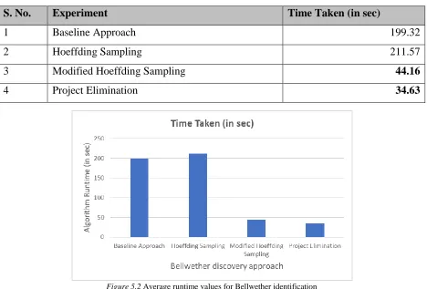
Table 5.2 Comparing run-times of all approaches for Bellwether identification
S. No. Experiment Time Taken (in sec)
1 Baseline Approach 199.32
2 Hoeffding Sampling 211.57
3 Modified Hoeffding Sampling 44.16
4 Project Elimination 34.63
Figure 5.2 Average runtime values for Bellwether identification
Table 5.3 Percentage of data required for training on a project and testing on others using Hoeffding bounds
Trained on
Tested on
ant camel ivy jedit log4j lucene poi velocity xalan xerces
ant - 5 6 7 8 9 10 11 12 13
camel 5 - 6 7 8 9 10 11 12 13
ivy 5 6 - 7 8 9 10 11.5 12 12.5
jedit 5 6 7 - 8 9 10 8 12.5 12
log4j 5 6 7 8 - 9 10 11 12 13
lucene 5 6 7 8 9 - 10 11 12 13
poi 5 6 7 8 9 10 - 11 12 13
velocity 5 6 7 8 7 10 11 - 12 13
xalan 5 6 7 8 8.5 10 11 12 - 13
28
RQ3: Does sampling data based on Hoeffding bounds outperforms idea of project
elimination?
All results were calculated after running for 30 iterations. Based on the values of average
run times in figure 5, it is evident that eliminating projects definitely reduces the time required for
finding bellwether project when compared with the baseline run time obtained by round robin
training of all projects against every other project. In addition to beating the run-time of the
baseline method, project elimination proved to be even better than sampling data using Hoeffding
bounds.
Table 1.4 Projects pruned during project elimination approach
Projects Eliminated
ant camel ivy jedit log4j
Table 5.5 G-Scores from project elimination approach
Project G-Score
Lucene 0.54
Poi 0.61
Velocity 0.49
Xalan 0.57
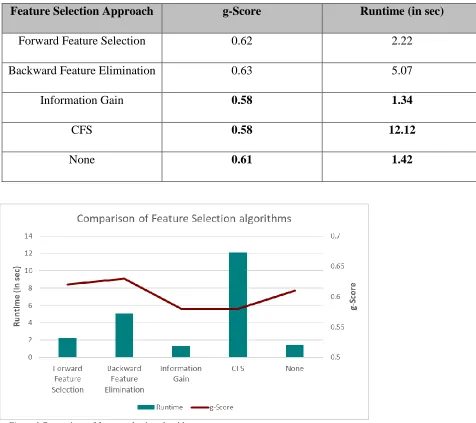
RQ4: Does feature selection improve the performance of the bellwether identification?
Among the feature selection algorithms implemented, information gain based feature
selection is the fastest while correlation-based feature selection is the slowest. Information gain
based feature selection is fastest because it calculates the information gain for all attributes before
starting with training the classifier and hence does not involve iterative training of a classifier
model. The results obtained using the inbuilt feature selection approach in Random Forest
29 still almost equivalent to the best feature selection algorithm results that require much more
computational time. Hence, it is better to go with the default feature selection in Random Forest
classifier rather than performing feature selection explicitly before training the model.
Table 5.6 Comparison of various feature selection algorithms for ‘poi’
Feature Selection Approach g-Score Runtime (in sec)
Forward Feature Selection 0.62 2.22
Backward Feature Elimination 0.63 5.07
Information Gain 0.58 1.34
CFS 0.58 12.12
None 0.61 1.42
30
CHAPTER 6: CONCLUSION Conclusion
In this thesis work, we have performed a thorough study of the Bellwether discovery
process and their importance in various software engineering domains. Our results show that we
can make the process of identification of bellwether project in a repository much faster than the
current round robin O(N2) approach.
We have shown that sampling the training and/or testing datasets helps in reducing the
amount of time spent on the bellwether discovery process. Data sampling not only helps to reduce
the run time of the code but also shows that efficiently selecting data from a project can help
minimize redundancies and ensure that the classifier is trained only on the optimum percentage of
training data. This comes at the almost negligible loss of the model performance measured using
g-score.
We also proved that sampling is not always the best method for reducing the time for
bellwether discovery. We can prune projects to avoid the time spent on training projects which are
highly unlikely to be prospective bellwethers. This helped to focus only on the projects that are
capable of being the representative project for the whole repository which essentially reduced the
runtime by some fraction of N, with N being the number of projects in the repository.
Finally, we also compared feature selection algorithms to improve the model performance
and reduce the time complexity of this process. But based results do not show any significant
improvement in model performance or reduction in runtime by incorporating these algorithms into
31
Future Work
Based on the results achieved in this project work, there are some more algorithms and
methods which can be explored to get even much better results. Some of the questions for which
more exploration can be done are discussed below.
1. Explore alternative sampling methods: Can we implement more sampling methods
instead of just Hoeffdings bounds and compare them? There is another sampling method named
Bayesian Races which assume that data is normally distributed. This approach might also prove to
be useful for reducing the time complexity associated with bellwether discovery.
2. Racing between the number of projects and sampling: Is it possible to determine which
approach needs to be taken sampling or elimination while just looking at dataset? Are there any
threshold values which help us determine we should either go for project elimination or sampling?
3. Exploring project elimination with sampling: In this work we focused on evaluating
sampling algorithms and eliminating projects in isolation. It would be interesting to see if we are
able to achieve even better results by combining the idea of project elimination and data sampling.
4. Exploring with different repositories: For the scope of this project, we limited ourselves
to the use of Jureczko repository, but we can explore more data set repositories and use them to
explore our research questions. It would help us to see how well our work applies to other
repositories.
5. Adding Parallelism to code: Another important aspect of computation is parallelism
built-in languages and platforms. Our current work does not explore this but adding parallelism to
32
REFERENCES
[1] Tim Menzies and Rahul Krishna, Bellwethers: A Baseline Method for Transfer Learning,
IEEE Transactions on Software Engineering, April 2018.
[2] Tim Menzies, Zhimin He, et. al., Learning from Open-Source Projects: An Empirical Study
on Defect Prediction, 2013 ACM / IEEE International Symposium on Empirical Software
Engineering and Measurement.
[3] Zhang, et. al., Software Analytics as a Learning Case in Practice: Approaches and
experiences, MALETS11, November 12, 2011, Lawrence, Kansas, USA.
[4] Sokolova, et. al., Beyond Accuracy, F-score and ROC: A Family of Discriminant Measures
for Performance Evaluation, 2006, American Association for Artificial Intelligence
(www.aaai.org).
[5] Shuo Wang and Xin Yao, Using Class Imbalance Learning for Software Defect Prediction,
IEEE TRANSACTIONS ON RELIABILITY, VOL. 62, NO. 2, JUNE 2013.
[6] T. J. McCabe, A complexity measure, Software Eng.,vol. 2, no. 4, pp. 308320, Feb. 1976.
[7] M.H.Halstead, Elements of Software Science,New York, NY, USA: Elsevier, 1977.
[8] T. Menzies, J. Greenwald, and A. Frank, Data mining static code attributes to learn defect
predictors, IEEE Trans. Software Eng., vol. 33, no. 1, pp. 213, Jan. 2007.
[9] C. Catal and B. Diri, Investigating the effect of dataset size, metrics sets, and feature
selection techniques on software fault prediction problem, Inf. Sci., vol. 179, no. 8, pp.
10401058, 2009.
[10] Y. Ma, L. Guo, and B. Cukic, A statistical framework for the prediction of fault-proneness,
33 [11] T. Hall, S. Beecham, D. Bowes, D. Gray, and S. Counsell, A systematic review of fault
prediction performance in software engineering, IEEE Trans. Software Eng., vol. 38, no. 6,
pp. 12761304, Nov.-Dec.2012.
[12] E. Arisholm, L. C. Briand, and E. B. Johannessen, A systematic and comprehensive
investigation of methods to build and evaluate fault prediction models, Syst. Software, vol.
83, no. 1, pp. 217, 2010.
[13] T. Menzies, B. Turhan, A. Bener, G. Gay, B. Cukic, and Y. Jiang, Implications of ceiling
effects in defect predictors, in Proc. 4th Int. Workshop Predictor Models Software Eng.
(PROMISE 08), 2008, pp. 4754.
[14] Tim Menzies, A. Dekhtyar, J. Distefano, and J. Greenwald, Problems with Precision: A
Response to Comments on Data Mining Static Code Attributes to Learn Defect Predictors,
IEEE Transactions on Software Engineering, vol. 33, Sepember 2007
[15] M. Kubat, S. Matwin et al., Addressing the curse of imbalanced training sets: one-sided
selection, ICML, vol. 97. Nashville, USA, 1997
[16] Maron, O., Moore, A.W., The Racing Algorithm: Model Selection for Lazy Learners,
Artificial Intelligence Review (1997) 11: 193.
[17] M. Jureczko and L. Madeyski, Towards identifying software project clusters with regard to
defect prediction, inProc. 6th Int. Conf. Predict. Model. Softw. Eng. -PROMISE 10. New
York, New York, USA: ACM Press, 2010, p. 1
[18] J. Novakovic, P. Strbac, D. Bulatovic., Toward Optimal Feature Selection using Ranking
Methods and Classification Algorithms, Yugoslav Journal of Operations Research 2011, No.
34 [19] M. A. Hall, G. Holmes, Benchmarking Attribute Selection Techniques for Discrete Class
Data Mining, IEEE Transactions on Knowledge and Data Engineering, Vol. 15, No. 3,
May/June 2003.
[20] F. Porto, L. Minku, E. Mendes, A. Simao, A Systematic Study of Cross-Project Defect
35
36
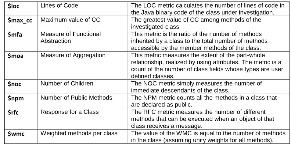
APPENDIX A Table A Data Dictionary [20]
Metric Notation
Metric Name Metric Description
$amc Average Method Complexity This metric measures the average method size for each
class. Size of a method is equal to the number of Java binary codes in the method.
$avg_cc Average of Cyclomatic
Complexity (CC)
CC is equal to number of different paths in a method (function) plus one. The McCabe cyclomatic complexity is defined as: CC=E-N+P; where E is the number of edges of the graph, N is the number of nodes of the graph, and P is the number of connected components. CC is the only method size metric. The constructed models make the class size predictions. Therefore, the metric had to be converted to a class size metric.
$ca Afferent Coupling The CA metric represents the number of classes that
depend upon the measured class.
$cam Cohesion Among Class
Methods
This metric computes the relatedness among methods of a class based upon the parameter list of the methods. The metric is computed using the summation of number of different types of method parameters in every method divided by a multiplication of number of different method parameter types in whole class and number of methods.
$cbm Coupling between Methods The metric measures the total number of new/redefined
methods to which all the inherited methods are coupled. There is a coupling when at least one of the conditions given in the IC metric is held.
$cbo Coupling between Object
Classes
The CBO metric represents the number of classes coupled to a given class (efferent couplings and afferent couplings).
$ce Efferent Couplings The CE metric represents the number of classes that the
measured class is depended upon.
$dam Data Access Metric This metric is the ratio of the number of private
(protected) attributes to the total number of attributes declared in the class.
$dit Depth of Inheritance Tree The DIT metric provides for each class a measure of the
inheritance levels from the object hierarchy top.
$ic Inheritance Coupling This metric provides the number of parent classes to which a given class is coupled. A class is coupled to its parent class if one of its inherited methods functionally dependent onthe new or redefined methods in the class.
$lcom Lack of cohesion in methods The LCOM metric counts the sets of methods in a class
that are not related through the sharing of some of the class fields.
$lcom3 Lack of cohesion in methods A low value of LCOM2 or LCOM3 indicates high cohesion
37
Table A (continued)
$loc Lines of Code The LOC metric calculates the number of lines of code in
the Java binary code of the class under investigation.
$max_cc Maximum value of CC The greatest value of CC among methods of the
investigated class.
$mfa Measure of Functional
Abstraction
This metric is the ratio of the number of methods inherited by a class to the total number of methods accessible by the member methods of the class.
$moa Measure of Aggregation This metric measures the extent of the part-whole
relationship, realized by using attributes. The metric is a count of the number of class fields whose types are user defined classes.
$noc Number of Children The NOC metric simply measures the number of
immediate descendants of the class.
$npm Number of Public Methods The NPM metric counts all the methods in a class that
are declared as public.
$rfc Response for a Class The RFC metric measures the number of different
methods that can be executed when an object of that class receives a message.
$wmc Weighted methods per class The value of the WMC is equal to the number of methods

![Table A Data Dictionary [20]](https://thumb-us.123doks.com/thumbv2/123dok_us/1774370.1228499/44.612.74.547.132.715/table-a-data-dictionary.webp)