International Journal of Emerging Technology and Advanced Engineering
Website: www.ijetae.com (ISSN 2250-2459, ISO 9001:2008 Certified Journal, Volume 6, Issue 1, January 2016)
102
Adaptive Observer Backstepping Control for Industrial Robot
Manipulators Using IMU
Tran Xuan Kien
1, Do Duc Hanh
21
R&D Department, Military Institute of Science and Technology, Hanoi, Vietnam 2Control Engineering Department, Military Technical Academy, Hanoi, Vietnam
Abstract—In this paper, an adaptive observer backstepping
control for robot manipulators in the presence of external disturbances and parametric uncertainties is developed. Only link angular positions are measured as outputs using an Inertial Measurement Unit (IMU) based on MEMS and Kalman Filter instead of encoders. A good performance of the designed control is achieved despite the presence of disturbances, parameter uncertainties, system nonlinearities and payload changes for a real-time system of a single-link flexible-joint manipulator.
Keywords—Adaptive Observer Backstepping, IMU, MEMS, Kalman Filter, Robot Manipulator Control.
I. INTRODUCTION
Backstepping is a systematic and recursive design methodology for nonlinear feedback control that breaks down the controller into steps and progressively stabilizes each subsystem (“step back” the feedback signals towards the control input) [1]. The backstepping method is used in numerous applications including robotic systems [4], [5]. Backstepping design provides a standard procedure to select Lyaponov function. Backstepping design procedure is based on the Lyapunov stability theory and applied for nonlinear systems with strict feedback form and adaptive to parameter uncertainties. A disadvantage of backstepping design procedure is that all states of the system must be measurable. For unmeasured states, an observer should be available to estimate. In this paper, an adaptive observer backstepping control is designed for nonlinear systems with parameter uncertainties, where only the output is measured and it is the only feedback for closed control loop, system nonlinearities are functions of the output. In the design procedure, the backstepping controller and observer are computed simultaneously. Update laws in the design procedure guarantee adaptability to parameter uncertainties.
The rest of the paper is structured as follows. In section II, an adaptive observer backstepping control design for a single-link flexible-join robot manipulator is presented. In section III we briefly introduce an Inertial Measurement Unit [2] and how it is installed and used instead of encoders to measure angular positions of the robot arm.
Experiment design and the performance of the designed real-time control for the flexible-joint robot arm with an IMU attached at the end of the robot arm and payload changes are presented in section IV. We conclude in section V.
II. ADAPTIVE OBSERVER BACKSTEPPING FOR SINGLE -LINK FLEXIBLE-JOINT ROBOT MANIPULATOR A. System Modeling
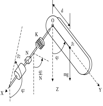
We consider a single-link flexible-joint robot manipulator actuated by a DC motor (see Fig. 1).
K
N
X Z Y
d
J1
J2
O
q2 q2 N
q1
mg
[image:1.612.348.515.378.551.2]Fig. 1. A single-link flexible robot manipulator
The dynamic equations of the system are as follows:
2
1 1 1 1 1 1
2
2 1 2 2 1
2
cos
0
t b
q
J q
F q
K q
mgd
q
N
q
K
J q
F q
q
K i
N
N
LDi
Ri
K q
u
(1)
International Journal of Emerging Technology and Advanced Engineering
Website: www.ijetae.com (ISSN 2250-2459, ISO 9001:2008 Certified Journal, Volume 6, Issue 1, January 2016)
103
The inertials J1, J2, the viscous friction constants F1, F2, the spring constant K, the torque constant K, the torque constant Kt, the back-emf constant Kb, the armature resistance R and inductance L, the link mass M, the position of link’s centre of gravity d, the gear ratio N and the acceleration of gravity g can all be unknown.B. The design procedure of adaptive observer backstepping control
We assume that only the link position q1 is measured.
The choice of state variables:
5
1
q
1,
2q
1,
3q
2,
4q
2,
i
The dynamic equations of the system become:
1 2
1 2
2 2 1
1 1 1
3 4
2 2
4 1 4 5
2 2 2
5 5 4
1
cos
1
t
b
mgd
F
K
y
J
J
J
N
K
F
K
J N
N
J
J
R
K
u
L
L
L
y
(2)
Clearly, (2) is not in the output-feedback. Differentiating y twice, we obtain
2
Dy
(D
d
dt
is the differentiation operator) and2 1 3
1 1 1
cos
mgd
F
K
D y
y
Dy
y
J
J
J
N
It implies that:
2
1 1
3
1 1 1
cos
J N
mgd
F
K
D y
y
Dy
y
K
J
J
J
3 2
1 1
4 3
1 1 1
cos
J N mgd F K
D D y D y D y Dy
K J J J
Differentiating and substituting
3,
4 , we obtain4 3 2
1 2 1 2 1 2
5 2
1 1 2 1 2 1 2
2 1 2
2 2
1 1 2 1 2 1 2 1 2
cos cos cos
J J N F F K K F F
D y D y D y
K K J J J J N J J
mgd F K F K mgd mgdK
D y Dy D y y
J J J N J J J J J J N
Finally, differentiating and substituting
5,
4 we arrive at the input-output description5 1 2 4 3
1 2 1 2 1
3
1 2 1 2
2
1 2 2 1 2 1 2
2
1 2 1 2 1
2 2
1 2 1 2 1 2 1 2 1 2
2 2
2 1
cos
cos
t
t b
t b
K K R F F mgd
D y u D y D y
J J NL L J J J
R F F K K K K F F D y L J J J L J J N J J
R K K F F F K F K K K F D y L J J N J J J J N J J J J L R F mgd
D y L J J
1 2
2
1 2 1 2 1 2 2
2 2
1 1 2
cos cos
t b
t b
R F K F K K K Dy L J J N J J J J L K RF K K mgd R mgd
D y y
N L L J L J J N
(3)
It is tedious but straightforward using (3) to find a choice of state variables.
1 2 1
2 3 2. 3.
3 4 4. 5.
4 5 6. 7.
5 0 8.
1
.
.cos .cos .cos . .cos
x x y
x x y y
x x y y
x x y y
x b u y y x
(4)
Where the unknown parameters
1
,
2,
3,...
8International Journal of Emerging Technology and Advanced Engineering
Website: www.ijetae.com (ISSN 2250-2459, ISO 9001:2008 Certified Journal, Volume 6, Issue 1, January 2016)
104
1 2
1 3 0
1 2 1 1 2
1 2 1 1 2
2 2
1 2 2 1 2 1 2
1 2 1 2 1
4 2 2
1 2 1 2 1 2 1 2 1 2
2 5 2 1 6 ; ; ; t t b b t
R F F mgd K
b
L J J J J J NL
R F F K K K K F F
L J J J L J J N J J
R K K F F F K F K K K F
L J J N J J J J N J J J J L
R F mgd
L J J
K R 1 2 2
1 2 1 2 1 2
2
7 2 8 2
1 2 1 2
; .
t b
t b
F K F K K K L J J N J J J J L K RF K K mgd R mgd
N L L J J L J J N
(5)
Hence, the design procedure of theorem is applicable to (4), and an adaptive controller that achieves bounded asymptotic position tracking from all initial conditions and for all position values of the constant J1, J2, F1, F2 K, Kt Kb, R, L.
We define new variables:
0
0
0 1 0 0 0 1
0
0 0 1 0 0 0
; 0 ; ;
0 0 0 1 0 0
0
0 0 0 0 1 0
0 0 0 0 0 0
A b c
b 8,5
0 0 0 0
0 0 0 0
0 cos 0 0 0
0 0 0 0
( )
0 0 cos 0 0
0 0 0 0
0 0 0 cos 0
0 0 0 0 cos
y y y y y y y y y
And rewrite (4) and (5) by using new defined variables as follows:
0
1
( )
( )
( )
p
j j m
j
x
Ax
y
y
b
y u
y
c x
(6)State-observers are designed as follows:
0
1 0
ˆ
.
.
p
j i j j
j j
x
b v
p = 8; m = 0
A0 is chosen so that
A
0A kc
is Hurwitz.1
2
0 3
4
5
1 0 0 0
0 1 0 0
0 0 1 0
0 0 0 1
0 0 0 0
k k A k k k
0 0 0 0 0 5.
( ) ( ), 1
j j j
j j e u
A ky y
A y j p
A
(7)
8
0 0
1
8 8
0 0 0
1 1
8
0 0 0 0
1 8
0 0 0
1 ( ) ( ) ( ) ( ) j j j
j j j j
j j
j j
j
j j j
j
v
Ax y bu bv
Ax y bu A ky y
A y bA bu
x
As
y
c x
T
Ax
ky
Ax
kc x
T
(
A
kc
T)
x
A x
08
0 0 0 0 0 0
1 8
0 0 0 0
1
j j
j
j j j
A A bA
A x b A
A x
It means that
x
x
is exponential and converges to zero since A0 is Hurwitz. Hence, virtual estimationx
ˆ
of x is:ˆ
0 1 0p j j j
x
b v
We are now ready to design our adaptive output-feedback controller.
International Journal of Emerging Technology and Advanced Engineering
Website: www.ijetae.com (ISSN 2250-2459, ISO 9001:2008 Certified Journal, Volume 6, Issue 1, January 2016)
105
1 r
( )
z
y
y t
(3.77)As
1 1 2 ,1
1
( )
pj j j
y
x
y
x
x
y
.The derivative of z1 is:
1 2 ,1
1
( )
pr j j r
j
z
y
y
x
y
y
Since x2 is not measured, it cannot be our virtual control.
We replace it with the sum of its “virtual estimate” and the corresponding error:
2 0,2 ,2 ,2
1 0
p m
j j j j
j j
x
b v
Substituting, we obtain
1 0,2 ,1 ,2 ,2
1 0
( )
p m
j j j j j r
j j
z
y
b v
y
with m = 0,
1
z
becomes:1 0,2 ,1 ,2 0,2
1
( )
p
j j j r
j
z
y
v
y
(8)The choice of virtual in (8) is v0,2because (7) reveals
that the control u appears in the 4th derivative of v0,2, sooner than for any of the other variables in (8). If v0,2 were the control and the parameters
1,
2,
3,...
8 were known, then our choice of control law would be0,2 1 1 1 1 0,2 ,1 ,2
1
.
( )
p
r j j j
j
v
c z
d z
y
y
1 1 1 1
.
1 0,2z
c z
d z
1 1 1 1 0,2 ,1 ,2 0,2
1
. ( )
p
r j j j
j
c z d z
y
y
v
1 1 1 1
.
1 2 0,2 0.
1 rz
c z
d z
v
y
We introduce the second error variable as
2 0,2 1 r
z
v
y
And substitute it into (8) we obtain
1 1 1 1 1 2 0
.
1 2 1z
c z
d z
z
0
1,
1 2... ...
81
1
c z
1 1d z
1.
1 02 0,1, 1,1 12,...
8,1 8,2,
v
0,2
Denoting the first estimate of
1 as
1, the first stabilizing function
1is chosen to be:1 1
.
1
(3.79) With this choice, the
1
z
- equation becomes
1 1 1 2 1
.
1 0 1.
1 2z
c z
z
d z
Our first Lyapunov function is
2 1
1 1 0 1 0 1 0
1
1
1
1
2
2
V
z
P
d
where
P
0
P
0 >0, satisfies0 0 0
.
01
P A
A P
The derivative of V1 is
0 1
1 1 1 0 1 1 0
1
1
.
d
V
z z
P
d dt
2 2
1 2 1 1 1 1 0 1 1 1 1 1 2
1
1
.
T.
.
z z
c z
d z
z
z
d
22 2
1 2 1 1 0 1 1 1 1 1 1
1 1
1
3
.
2
4
T
z z
c z
z
d z
d
d
(10)
The
0 1
-term is now eliminated from (10) by the choice of update law
1 1 1
z
(11) which yields2
1 1 2 1 1
1
3
.
.
4.
V
z z
c z
d
Step 2: The derivative of
2 0,2 1 r
z
v
y
is expressed as2 0,2 1 r
z
v
y
1
2 0,1 0,3 0,2 2 2
1
.
.
,
k v
v
y
y
y
International Journal of Emerging Technology and Advanced Engineering
Website: www.ijetae.com (ISSN 2250-2459, ISO 9001:2008 Certified Journal, Volume 6, Issue 1, January 2016)
106
0 1 1 10 0 0 2 0 0
0
1 1 1
0 1 1
0 1
.
.
( )
.
( )
.
i p i j j i mi r r
j
i r
A
k y
y
A
y
A v
z
y
y
v
y
where
0,2 1 ,1 ,2 0,2
p
j j j j
y
y
1 1 1
z
1,
2,
3..., ... , 1
8
T
1
2 1,1 12
,...,
8,1 8,2,
0,2T
v
y
Using the estimate2
of2
, the stabilizing function2
is defined:
2 1 12 2 2 1 2 2 2 0,1 0,2 0,1
1 1
2 2 0 0 0 0 0
0 0
1 1 1
0 0 1 1
1
.
.
.
.
.
p T i j i mj i r
i r
c z
z
d
z
k v
y
y
y
A
k y
y
A
y
A v
z
y
v
y
And from definition
z
3
v
0,3
2
y
rwe rewrite this equation as
2
1 1
2 2 2 1 2
.
.
2 2 3 2 2z
c z
z
d
z
z
y
y
The derivative of the nonnegative function V2
2 1
2 1 2 2 2 0
2
1
1
1
2
2
V
V
z
P
d
is computed as
2 1 2 2 2 2 0
2
1
.
d
V
V
z z
P
d dt
2 2
1 2 1 1 2 2 1 2 2 3
1
3
.
.
.
4
z z
c z
c z
z z
z z
d
1 2 2 1
2 2 2 2 2 2 02 2
2
1
.
.
.
T
z
d
z
z
y
y
d
2 22 3 1 1 2 2
1
3
.
4
z z
c z
c z
d
1 2 22 2 2 2 2 2
2 2
1
3
2
4.
T
z
d
z
y
d
d
2 22 3 1 1 2 2
1 2
2 2 2 2
3
3
.
4
4
T
z z
c z
c z
d
d
z
The
2
- term is then eliminated with the update law
2 2 2
z
(13) which yields2 2
2 2 2 1 1 2 3
1 2
3 1
1
.
.
4
V
c z
c z
z z
d
d
Step 3: from definition
3 0,3 2 r
z
v
y
the derivative ofz
3is expressed as
z
3
v
0,3
2
y
r2
3 0,1 0,4 02 2 3
2 .y y
k v
v
y
2 20 0 0 0
0
0
.
.
pj.
i ji
i
k y
y
y
2 2 2 2
0 0 1 1 2 2
1 2
1 2
.
m
j j r r
i r
v
z
z
y
y
v
y
where1 1 1
z
;
1,
2,
3, ... , 1
8
2
3 1,1 1,2
,...,
8,1 8,2,
v
0,2y
International Journal of Emerging Technology and Advanced Engineering
Website: www.ijetae.com (ISSN 2250-2459, ISO 9001:2008 Certified Journal, Volume 6, Issue 1, January 2016)
107
2 2 23 3 3 2 3 3 3 0,1 02 0.1
2 2
3 3 0 0 0 0
0 0
.
.
.
p i i j ic z
z
d
z
k v
y
y
y
k y
y
y
2 2 2 2
0 1 1 2 2
0 1 2
1 2
.
m
i r
j i r
v
z
z
y
v
y
And definition
4 0,4 3 r
z
v
y
we rewrite this equation as
2
2 2
3 3 3 2 3
.
.
3 2 4 3.
3T
z
c z
z
d
z
z
y
y
The derivative of the nonnegative function
2 1
3 2 3 3 3 0
3
1
1
1
2
2
V
V
z
P
d
is computed and
2 2 2
3 2 3 1 1 2 2 3 3 2 3 3 4
1
3
.
.
4.
V
z z
c z
c z
c z
z z
z z
d
2 2 23 3 3 3 3 3
3 3 2
1
1
1
.
2.
4.
T
z
d
z
y
d
d
d
2 2 2
3 4 1 1 2 2 3 3
1 2
3
3
.
.
.
4.
4.
z z
c z
c z
c z
d
d
2 2 23 3 3 3 3 3
3 3
1
3
2.
4.
T
z
d
z
y
d
d
2 2 2
3 4 1 1 2 2 3 3
1 2 3
3 3 3 3
3
3
3
.
.
4
4
4
T
z z
c z
c z
c z
d
d
d
z
The
3
- term is then eliminated with the update law
3 3
z
3
(14) which yields2 2 2
3 3 3 2 2 1 1 3 4
1 2 3
3 1
1
1
.
.
.
.
4
V
c z
c z
c z
z z
d
d
d
Step 4: From definition
z
4
x
4
y
(3)r
3 the derivative ofz
4 is expressed as
0
1 2 3
0 0
0 0 0 0 0
0 0
4 4
4 0,4 3 4 0,1 0,5 02 2 5
4
3 3 3 3
1 1 2 2 3 3
1 2 3
.
.
.
.
i p i j j r r r rA
k y
y
A
y
z
v
y
k v
v
y
z
z
z
y
y
y
where: 34 1,1 12
,...,
8,1 8,2,
v
0,2y
(3.87)Denoting the first estimate
as4
the 4th stabilizing function
4 is chosen to be
1 2 3
2
3 3
4 4 4 3 4 4 4 0,1 02 0,1
3 3
4 4 0 0 0 0
0 0
3 3 3 3 3
0 1 1 2 2 3 3
0
1 2 3
.
.
.
.
.
p i j j i m i r j i rc z
z
d
z
k v
y
y
y
A
k y
y
A
y
A v
z
z
z
y
v
y
And definition
z
5
v
0,5
4
y
r 4 we rewrite this equation as
2
3 3
4 4 4 3 4
.
.
4 2 5 4.
4T
z
c z
z
d
z
z
y
y
The derivative of the nonnegative function
2 1
4 3 4 4 4 0
4
1
1
1
2
2
V
V
z
P
d
is computed and
2 2 2
4 4 3 1 1 2 2 3 3
1 2 3 4
2
2 3 2
4 4 4 3 4 5 4 4 4 4 4 4
3 1
1
1
1
.
.
4
.
.
T
V
z z
c z
c z
c z
d
d
d
d
c z
z z
z z
z
d
z
y
2 2 2 2
1 1 2 2 3 3 4 4
1 2 3 4
3 1
1
1
1
.
4
c z
c z
c z
c z
d
d
d
d
International Journal of Emerging Technology and Advanced Engineering
Website: www.ijetae.com (ISSN 2250-2459, ISO 9001:2008 Certified Journal, Volume 6, Issue 1, January 2016)
108
3 2 24 4 4 4 4 4
4 4 4
1
1
1
.
2
4.
T
z
d
z
y
d
d
d
2 2 2 2
1 1 2 2 3 3 4 4
1 2 3 4
4 4 4 4
3 1
1
1
1
.
4
T
c z
c z
c z
c z
d
d
d
d
z
The
4
- term is then eliminated with the update law :4 4
z
4
(15) which yields2 2 2 2
4 4 4 3 3 2 2 1 1
1 2 3 4
3 1
1
1
1
.
4
V
c z
c z
c z
c z
d
d
d
d
Step 5: From definition (5)
5 0,5 4 5
z
v
y
the derivative of5
z is expressed as
(5)
5 0,5 4 5
z
v
y
4 4
5 0,1 02 2 5
,
.
y y
k v
u
y
01 2 3
4 4
0 0 0 0 0
1
(5)
4 4 4 4 4
1 1 2 2 3 3 4 4
1 2 3 4 4
.
( )
.
( )
i p i j j r r rA
ky
y
A
y
y
z
z
z
z
y
y
y
where
1,
2,
3, ... ...
8, 1
4
5 1,1 12
,...,
8,1 8,2,
v
0,2y
Denoting the first estimate
as5
the control is thus chosen as
1 2 3
2
4 4
5 5 4 5 5 5 0,1 02 0,1 5 5
4 4 4
0 0 0 0 0
0 1
4 4 4 4 4
0 1 1 2 2 3 3 4 4
0
1 2 3 4
. ( )
. . ( ) . ( )
.
p
i j r
j i m i j i
u c z z d z k v y
y y
A k y y A y y
y
A v z z z z
v
(16)The derivative of the nonnegative function
2 1
5 4 5 5 5 0
5
1
1
1
2
2
V
V
z
P
d
is computed and
2 5 4 5 1 1
1 2 3 4
2 2 2 2
2 2 3 3 4 4 5 5 4 5 5 5 5 5
2 2
4 4
5 5 5
5
3 1 1 1 1
. .
4
1
. . . .
T
V z z c z
d d d d
c z c z c z c z z z z
d z z
y y d
2 2 2 2
1 1 2 2 3 3 4 4
1 2 3 4
5 5 5 5
3 1 1 1 1 . 4
T
c z c z c z c z
d d d d z
2 2 2 2 2
1 1 2 2 3 3 4 4 5 5
1 2 3 4
2
2 4
5 5 5 5 5 5
5 5 5
3 1
1
1
1
.
4
1
1
1
.
2
4.
T
c z
c z
c z
c z
c z
d
d
d
d
z
d
z
y
d
d
d
2 2 2 2
1 1 2 2 3 3 4 4
1 2 3 4
3 1
1
1
1
.
4
c z
c z
c z
c z
d
d
d
d
5
5 5 5
T
z
The
5
- term is then eliminated with the update law:
5 5
z
5International Journal of Emerging Technology and Advanced Engineering
Website: www.ijetae.com (ISSN 2250-2459, ISO 9001:2008 Certified Journal, Volume 6, Issue 1, January 2016)
109
which yields2 2 2 2 2
5 5 5 4 4 3 3 2 2 1 1
1 2 3 4
3 1
1
1
1
.
4
V
c z
c z
c z
c z
c z
d
d
d
d
is rendered nonpositive:
5 2 5
1
3
.
.
4
i i i
i
V
c z
d
(18)Stability and convergence. Due to the piecewise continuity of ( )
( )
p r
y t and the smoothness of the
nonlinearities (4), the solution of the closed-loop adaptive system exists. Let its maximum interval of existence be [0,tf). On this interval, the nonnegative function V5 is nonincreasing because of (18). Thus
1
, ,... , ,
2 5 1 2,...
5z z
z
are bounded on [0,tf) by constantsdepending only on the initial conditions of adaptive system. Moreover
0
A
shows that is bounded. The boundedness of all other signals on [0,tf) is established too.Since
1
z and yr are bounded, it follows y is bounded.
III. USING AN IMUINSTEAD OF ENCODERS TO MEASURE
ANGULAR POSITIONS
Development and implementation of an Inertial Measurement Unit (IMU) to estimate the attitude of objects in space is introduced in [2], [3]. Micro-Electro-Mechanical System (MEMS) sensors are used to measure angular velocity and acceleration, a magnetic sensor (magnetometer) is used to calibrate against orientation drift, a GPS signal receiver is integrated and an extended Kalman filter algorithm is applied for real time signal processing. To measure angular positions of the robot arm, a small and low-cost IMU is used instead of absolute encoders for installation convenience but ensures the required accuracy. Attachment and installation of encoders in the shaft of the robot arm is not easy. The IMU is attached at the end of the robot arm. It can actually be placed anywhere in the robot arm and needs no link to the shaft. Due to space limitations, we skip the detailed IMU implementation in this paper.
IV. EXPERIMENT DESIGN A. Experiment and simulation setup
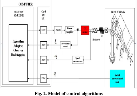
[image:8.612.324.563.313.480.2]A 2-DOF flexible-joint robot arm control is implemented based on algorithms shown in section II and using an IMU described in section III to measure angular positions. The control algorithms are modelled in Simulink, run in real-time under Real Time Window Target utility of Real Time Workshop, and interface through a PCI1711 card from Advantech with the real world robot arm (see Fig. 2). This model consisted of MATLAB/Simulink algorithm, PCI1711 card, DC motor with PWM driver and IMU. Torque transmission between the actuator (DC motor) and the plant (industrial robot arm) is of spring drive as a flexible-joint.
Fig. 2. Model of control algorithms
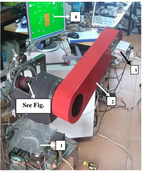
To investigate the proposed control algorithms, we designed an industrial robot arm model, as depicted in Fig. 3, where
1- PWM driver and power amplifier 2- Industrial robot arm
3- Inertial Measurement Unit
International Journal of Emerging Technology and Advanced Engineering
Website: www.ijetae.com (ISSN 2250-2459, ISO 9001:2008 Certified Journal, Volume 6, Issue 1, January 2016)
[image:9.612.332.548.120.313.2]110
Fig. 3. Industrial robot arm’s and hardware implementation Fig. 4 shows DC motor, gear and spring-based joint, where:
1- DC motor 2- Spring-based joint
3- Industrial robot arm’s gear.
Fig. 4. DC motor, gear and spring-based joint B. Simulation Enviroment
Matlab/Simulink has been used to simulate the proposed algorithms. Then, the simulated algorithms are implemented in a real-time hardware using Real-time Workshop with DAQ cards.
The Simulation model is built using normal Simulink blocks. States, signals, and model parameters can be viewed, modified in run-time. That allows to find an optimal control parameter set, and controller types as well.
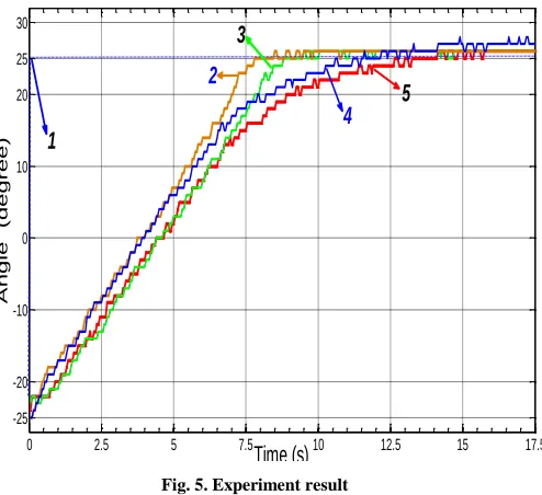
The experiment result is shown in Fig. 5, where line 1 depicts the setpoint (for robot arm angle) change from -25o to +25o. The other lines show changes of the robot arm angle output signals for different controllers, namely:
2- adaptive observer backstepping+PID without payload
3- adaptive observer backstepping + PID with payload 4- PID without payload
5- PID with payload.
2
1 3
4
1
3
See Fig.
4
[image:9.612.48.293.132.429.2]International Journal of Emerging Technology and Advanced Engineering
Website: www.ijetae.com (ISSN 2250-2459, ISO 9001:2008 Certified Journal, Volume 6, Issue 1, January 2016)
111
0 2.5 5 7.5 10 12.5 15 17.5
-20 -10 0 10 20 30
-25 25
Time (s)
A
n
g
le
(
d
e
g
r
e
e
)
4
5
2
3
[image:10.612.52.299.139.365.2]1
Fig. 5. Experiment result
The result shows that control and adaptability laws (11) (13), (14), (15), (17) from the proposed adaptive observer backstepping algorithms in section II ensure the stability and adaptability despite parameter uncertainties in the system. Using adaptive observer backstepping control algorithm combined with PID, the robot arm’s angle closely tracks the setpoint with static error 1o, response time 08s, while static error and response time are 2o and 11s for PID control respectively. In the experiment, even though the payload is three times heavier than the arm robot, the performance of the adaptive observer backstepping controller is almost unchanged (with static error 1o and response time 08s) and that proves the adaptability of the proposed control algorithms.
V. CONCLUSIONS
In this paper, an adaptive observer backstepping control for robot manipulators is developed. Only link angular positions are measured as outputs using a low-cost IMU based on MEMS and Kalman filter instead of encoders for easy installation but no accuracy suffering. The stability and good performance is achieved despite the presence of disturbances, parameter uncertainties, system nonlinearities and payload changes. The result is shown for a real-time system of a single-link flexible-joint manipulator, but the proposed algorithms can be extended and applied to more complex industrial robot manipulators.
REFERENCES
[1] M. Krstic, I. Kanellakopoulos, P. Kokotovic, Nonlinear and Adaptive Control Design, Wiley, 1995.
[2] B. H. Hue, T. X. Kien, D. M. Dinh, D. D. Hanh, “Model-based Development and Implementation of Real-time Object Spatial Attitude Estimation”, International Journal of Computer and Electrical Engineering (IJCEE), Vol. 5, No. 4, pp. 372-377, 2013. [3] B. H. Hue, N. N. Hung, T. X. Kien, D. D. Hanh, D. M. Dinh,
“Calibration against Orientation Drifts in a Real-time Embedded Inertial Measurement Unit”, International Conference on Computing, Management and Telecommunications (ComManTel), 2014
[4] Bo Zhou, “Backstepping Based Global Exponential Stabilizaton of a Tracked Mobile Robot with Slipping Pertubation”, Journal of Bionic Engineering, 2011, 8:69-76.