A singular perturbation method of calculating the behavior of supercavitating hydrofoils with rounded noses

HYDROFOILS WITH ROUNDED NOSES

Thesis by

Okitsugu Furuya

In Partial Fulfillment of th.e Requirements For the Degree of

Doctor of Philosophy

California Institute of Technology Pasadena, California

1972

ACKNOWLEDGMENT

I wish to thank my research advisor, Professor Allan J. Acosta, for his most generous guidance and encouragement during my years of graduate study at the California Institute of Technology. Specifically, his recognition of the importance of this type of problem and his unique suggestions on the approach have made it possible to accomplish the present work. I also thank him for the opportunities given to me to present this subject on many occasions.

I would also like to acknowledge Professor Theodore Y. T. Wu for his interest in the present problem, and particularly for his useful suggestions on the numerical procedure of his own work which has been used for comparison with the present work.

I am grateful to the Institute for four years of tuition payments and financial assistance for me and my family. This work was sup-ported partially by the Office of Naval Research and a major part of the computing was done under an Institute grant. This help is gratefully acknowledged.

Thanks are due to Mrs. Julie Powell and Mrs. Lynne Lacy for the competent typing and careful preparation of the manuscript under the pressure of shortage of time.

ABSTRACT

A simple, direct and accurate method to predict the pressure distribution on supercavitating hydrofoils with rounded noses is

presented. The thickness of body and cavity is assumed to be small. The method adopted in the present work is that of singular perturbation theory. Far from the leading edge linearized free streamline theory is applied. Near the leading edge, however, where singularities of the linearized theory occur, a non-linear local solution is employed. The two unknown parameters which characterize this local solution are determined by a matching procedure. A uniformly valid solution is then constructed with the aid of the singular perturbation approach.

The present work is divided into two parts. In Part I isolated supercavitating hydrofoils of arbitrary profile shape with parabolic noses are investigated by the present method and its results are com-pared with the new computational results made with Wu and Wang's exact "functional iterative" method. The agreement is very good. In Part II this method is applied to a linear cascade of such hydrofoils with elliptic noses. A number of cases are worked out over a range of cascade parameters from which a good idea of the behavior of this type of important flow configuration is .obtained.

Some of the computational aspects of Wu and Wang's functional iterative method heretofore not successfully applied to this type of

· TABLE OF CONTENTS

ACKNOWLEDGMENT ABSTRACT

TABLE OF CONTENTS NOMENCLATURE INTRODUCTION

PART I. ISOLATED SUPERCAVITATING HYDROFOILS WITH ROUNDED NOSES

1. Statement of the Problem 2. Outer Solution

3. Inner Solution 3. 1 Regular Case 3. 2 Critical Case 4. Matching

4. 1 Expansion of the Outer Solution 4. 2 Expansion of the Inner Solution 4. 3 Matching for the Regular Case 4. 4 Matching for the Critical Case

5. Construction of Uniformly Valid Solutions 5. 1 Uniformly Valid Solutions for the

Regular Case

5. 2 Uniformly Valid Solutions for the Critical Case

6. Special Cases

6.

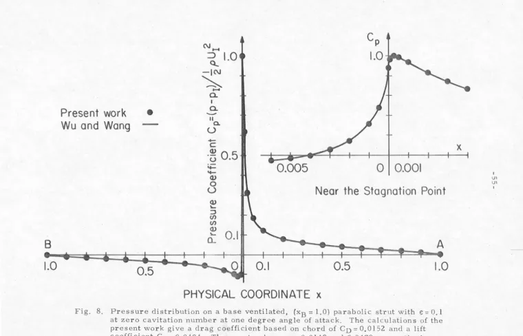
1 Infinite Cavity Case for an Arbitrary Profile Shape with a Parabolic Nose 6. 2 Parabolic Strut at Zero Cavitation

6. 3 Base-Vented Parabolic Strut 7. Numerical Results and Discussion 8. Sununary

References

List of Figure Captions Appendices

PART II. LINEAR CASCADES OF SUPERCAVITATING HYDROFOILS WITH ROUNDED NOSES

1. Statement of the Problem 2. Outer Solution

3. Inner Solution 4. Matching

5. Uniformly Valid Solutions

6. Numerical Calculations and Dis~us sions 7. Summary

References

Li st of Figure Captions Appendix

41 41 44 45 47 65

NOMENCLATURE

A lower separation point of cavity B upper separation point of cavity

c

connection point between rounded nose and arbitrary profile

shape

CL lift coefficient based on the chord length normalized by the dynamic pressure on the cavity in the direction normal to the upstream flow

CD drag coefficient based on the chord length normalized by the dynamic pressure on the cavity in the direction of the

upstrea1n flow

lift coefficient defined in the same way as CL but in the direction normal to the vector mean of the inlet and outlet velocity vector

drag coefficient defined in the same way as CD but in the direction of the vector mean

cp pressure coefficient defined by (p-pI)

Ii

p

ui

C pressure coefficient defined by (pp )/

-2 1

pU2, C

=

C for

Pc c c p Pc

d

F(()

H(C) £

(J

=

0.

space of hydrofoils in linear cascade

p q. 1 u v u n v n

u u nE:' nCY

v v nE:' nCY

w(z}

W(C)

u.

1

pressure

cavity pres sure

a rational function

velocity distribution in the inner region velocity distribution in the outer region stagnation point

velocity component in the x-direction

velocity component in the y-direction

normalized velocity component of the

n~

order in € only

in the x-direction

normalized velocity component of the

n~

order in € only

in the y-direction

normalized velocity components of the

n~

order in € and

CY respectively in the x-direction

normalized velocity components of the n

~

order in € and CY respectively in the y-direction

complex velocity potential in the physical plane complex velocity potential defined by iw(z) in the

transform plane

magnitude of the local uniform flow speed in the inner region

magnitudes of the flow speed at upstream and downstream

infinity, respectively

U

00 vector mean of the vectors Ur and UII

Uc velocity on the cavity ( = Ur

....fT+CJ)

X,Y

coordinates in the inner region

z complex variable in the linearized physical plane

z

complex variable in the inner region

flow angles at upstream and downstream infinity, rewritten

by E:

6r

and E:6II, respectively

aB geometrical angle between hydrofoil chord and 5r-axis

a

angle of the body axis with the x-axis (= e:

c )

c c

a

00 flow angle of the vector mean Y stagger angle

·../' geometric stagger angle used in fully wetted linear cascade

r

61' 611' 6 c E:

(, rt

e

A.,

µ;

i;, T)

w

theory, defined by Y - Cle -ClB in the present work contour used for contour integrals

see a

1, all and ac

small quantity in linearized theory transform planes

flow angle

coordinates in

x.

and ( planes respectively

cavitation m.nnber based on the upstream pressure, defined 1 2

by (Pr - Pc)

I

2

PU I

INTRODUCTION

Long cavitites are often created downstream of vane sections in pumps, turbines and on the components of the modern high speed hydrofoil craft. In order to maintain mechanical strength such supercavitating hydrofoils necessarily have rounded or locally blunt leading edges. It is this feature that poses difficult problems for analysis. Because of the roundedness or bluntness, the location of the cavity separation on the suction side of the lifting body is

com-pletely unknown. Therefore, it is important to predict not only the forces but also the pressure distribution on the body, since the latter may possibly indicate the separation point of the cavity on the curved

surface.

There exist various methods of attacking free streamline problems of the type associated with hydrofoils. These are the full non-linear theory and a later linearized free streamline method

purpose. But in actual computations with this method numerical complexities and difficulties often arise. The most troublesome aspect is computational instability which seems to be inherent in this type of problem. For example, Lurye [15] who applied Wu and Wang's method to base-vented parabolic struts was unable to obtain convergent solutions.

Many attempts have been made to avoid the non-linearity of the exact theory and also its computational difficulties. Brodetsky, Oba, Larock and Street, and Murai and Kinoe [4, 5, 6, 7 respectively] expressed the flow angle on the bcidy by power series in the potential. Larock and Street took only two such terms, while Murai and Kinoe incorporated leading edge curvature in these power series expansions. The coefficients in these power series are obtained by collocation of the flow angle or curvature on the body at discrete points. The final profile found as the result of calculation cannot be determined in advance unless a very great number of terms in the series are used.

On the other hand the linearized free streamline theory of Tulin [8] is a simple and direct theory which is useful for the calcu-lation of the forces on thin bodies. Yet this theory fails to predict the pressure on the body except far away from the leading edge, because such linearized theories require singularities at the leading edge to represent the stagnation flow there.

The method adopted in the present work for this purpose is

that of singular perturbation theory as described in the books by

Van Dyke [10] and Cole [11

J.

In what follows we describe the basic

idea of the new application of this theory to the present problem.

Assume that the angle of attack, camber and body- and

cavity-thickness are all sufficiently 11 _{small". Far from the leading edge}

(called here the "outer region") the perturbed velocities are considered

to be small in respect to the undisturbed flow so that linearized free

streamline theory can be applied. In terms of this perturbed complex

velocity, one can reduce the problem to a mixed-type Hilbert boundary

value problem which has been thoroughly treated by Muskhelishvili [12].

Near the leading edge of the foil the curvature of the surface is

large and generally there is a stagnation point nearby. This is the

region of the flow which in the parlance of the singular perturbation

literature is called the "inner region". In this portion of the flow the

linearized theory is not applicable and in fact the local solution in this

region is very non-linear with the local velocities differing greatly in

magnitude and direction from the free stream velocity.

The flow in this nose region past supercavitating hydrofoils may

be very complex. The flow past a simple supercavitating flat plate,

for example, exhibits a forward facing streamline which has infinite

curvature at the detachment point which decays as arc length to the

inverse fourth power. The distance of the stagnation point from the

leading edge in such a flow is proportional to the fourth power of the

flow may be fully wetted near the nose; base vented or cavitating profiles are an example of this type of configuration. However it may happen that a free streamline (arising either from cavitation or venti-lation) may originate near the leading edge. In this case the cavitation separation may be of two types (as discussed in the literature cited thus far); these are a 1'fixed detachment 11 point or a 1'smooth detach-ment1'. In the former the pressure gradient on the body becomes infinite on the wetted body at the detachment point and the curvature of the ensuing free streamline is infinite at this point. The smooth separation exhibits zero pressure gradient at detachment and the radius of curvature of the free streamline there matches that of the body.

this kind of application. Both cavitation and ventilation occur on bodies

having smooth, rounded leading edges; the position of this type of

separation or detachment is not fixed in advance. It depends upon the

local viscous flow, surface tension, and other physical parameters of

the flow and as of this date cannot be predicted, but must be measured.

The present work, as will be seen, is still applicable to this situation

provided the separation point is known. It should be mentioned that

all of the "exact" theories suffer the same degree of uncertainty in

regard to free streamline detachment on smooth bodies. It follows

that the criterion of 11

smooth" separation referred to before does not

necessarily mean that this type of free streamline separation actually

occurs,011 bodies in real fluids. A full discussion of this as yet

unresolved problem is beyond the scope of the present work. It is

brought up here only to note that in what follows the separation point

will be fixed a priori. Whether such a point coincides with a free

streamline 11 _{smooth" separation point on a continuous body must, as}

of this writing, be decided by experiment.

From the foregoing discussion it can be perceived that the local

flow around the nose will fall into two classes. In the fir st, the local

flow is fully wetted because in this case the free streamline separation

is well downstream. In this situation the 11_{inner flow" is that around}

a semi-infinite half body which has the coordinates of the nose region

of the body. This type of problem is a standard one in fluid mechanics

and is readily solved by two-dimensional potential flow methods. In

the present work this is called the 11_{regular case}11

• As will be shown,

with are unknown. The second class as might be surmised exhibits a free streamline within the inner region. This considerably complicates the inner flow because (just as in the full non-linear treatment) the exact position of this streamline is unknown in advance. However,

. an "exact" knowledge of this inner streamline would exceed the

expectations originally laid out for the present work. To recapitulate, we hope to find a solution for the set problem everywhere as accurate as the linear solution where the linear solution itself is appropriate. We do not therefore need an "exact" inner solution when a free streamline is present there, and, as will be seen, a sufficiently

accurate solution can be obtained by a simple assumption. This class of inner problem, when the inner solution contains a free streamline, is termed herein a 11

critical case".

Thus far no assumption has yet been made about the shape of the nose region itself. Insofar as the present method goes it can be arbitrary. Nevertheless, there is a considerable advantage in keeping the inner solution as simple as possible. The reasons for this will become evident in the section to follow. A particularly simple nose section is that of a parabola. In fact most airfoil and hydrofoil profiles have leading edges reasonably well approximated by parabolas, and this shape possesses attractively simple, explicit formulations of the surrounding flow field. This leading edge profile is therefore adopted in the pre sent work as being expeditious and practical but by no

means is the methodology to be expounded limited to it.

As mentioned, two parameters in the inner flow past the

magnitude of the local uniform flow speed and the location of the

stagnation point of the flow about the parabola. These quantities are

determined by 11_{matching procedure}11 _{of the singular perturbation} method in such a way that the local 11_nose11 _{solution (or inner solution)}

blends smoothly into the linear solution far away from the nose (or

outer solution) with the error never exceeding that of each of its

constituent solutions.

The singular perturbation method is completed by constructing

a uniformly valid solution out of the two obtained solutions, inner and outer. The simplest method of doing this is to add the inner and outer

solution and to subtract the part they have in common. In this process

the deficiencies of the linearized theory are removed by eliminating

its singularities.

In the present work only two-term outer and one-term inner

expansions have been used.

In the first part of this thesis we show the mathematical basis

of the singular perturbation method, using simple flow profiles for isolated supercavitating hydrofoils and with those sections prove the validity and accuracy of this method by comparison with an exact theory.

The profile used is that of an isolated supercavitating parabolic wedge.

This work is then extended to account for an arbitrary camber function

downstream of the parabolic nose and for non-zero cavitation number.

In Part II of this thesis the present method has been applied to

Although the nose shape is changed to that of an ellipse, it still has a

parabolic nose locally as mentioned earlier. Therefore the inner

solu-tions remain exactly the same as those in Part I.

Linearized free streamline theory should be carefully applied

to find outer solutions when it is used for cascade problems. Since the

flow is turned or deflected through the cascade, the relevant

perturba-tion of the velocities should be made in respect to the vector mean of

the inlet and outlet velocity, and at the same time the vector mean

should be correctly aligned with the linearized flow configuration so

that a consistent representation within the framework of the linearized

theory is carried out. This point has escaped many workers using

linearized free streamline theories for linear cascade problems in the

recent past as will be discussed later. The many parameters and the

variable flow geometry make the computation of cascade flows very

tedious. Nevertheless as will be shown these cases can be treated

with only somewhat more complexity than for isolated hydrofoils. In

the numerical work on these flows profile shapes consisting of an

ellip-tical forebody connected to a straight line and a circular arc after

profile were used. These kinds of profiles resemble (except for the

leading edge thickness) supercavitating propeller sections now in use.

They exhibit surprisingly good lift-to-drag ratios for the circular arc

PART I

ISOLATED SUPERCAVITATING HYDROFOILS

WITH ROUNDED NOSES

1. Statement of the Problem. Consider a flow configuration of an

isolated supercavitating hydrofoil as shown in Fig. 1, assuming two

dimensional, incompressible potential flow. The rounded nose of the

hydrofoil is defined by a parabola y

=

±

e/X,

E: being a small parameter.

The lower side of the nose is smoothly connected to an arbitrary

pro-file shape of y

=

8h(x) at a point denoted by "C" (x

=

x ). The point ''C" c

is arbitrary but assumed to be located sufficiently far away from the

leading edge in this method. We also assume that a cavity detaches at

two points; namely, at A and Bon the body. The separation is fixed

but arbitrary and extends downstream the distance

"

£"

.

The pres sure

p in the cavity is assumed to be constant. Therefore we can define a

c

pressure coefficient normalized by the dynamic pressure on the cavity

by

( 1)

and cavitation number by

Ci

=

(2)

where p

number

er

is also assumed to be small and of the same order as e:. The

flow approaches the body at a small angle

°J

with x-axis, which is

rewritten by e:

o

1 for notational convenience.

With the flow model as stated above we proceed now to consider

a regular perturbation method, namely, linearized free streamline theory of Tulin [8] to find the outer solution.

In our particular small perturbation problem there are two

small parameters which control the perturbations rather than one. These are e: and

er,

and they are independent. We now obtain in the usual way perturbation expansions in terms of these variables, i. e. ,

u

u

(3a)

c

(3b)

where

( 4)

using the Bernoulli equation. With the original form in mind une: and

uncr' and vne: and vncr are combined to rewrite Eqs. (3a) and (3b) as

follows

u

u

_c (3a')

v 2

U

=

e:v 1

+

e:

v 2

+ · · ·

(3

b')

c

where

The complex velocity potential w can be defined by

w

u

_c = u-iv

u

_c

2 = 1

+

ew

1

+

€ w 2

+ ...

wn

=

(u - iv )/U

n n c

( 5)

(6)

( 7)

(8)

(9)

The term w

1 is that of the fully linearized free streamline theory. It is regular and uniform far from the leading edge, but it is singular

near the leading edge, because the assumption of small disturbances

around the stagnation point is violated there. Since the regular

pertur-bation theory breaks down near a stagnation point, the idea of a

singu-lar perturbation theory becomes relevant.

The first step for this theory is to find a local non-linear

solution in the region where the singularities of the linearized theory

are located. This "inner" region can be easily found from the nature

of singularities in the outer solution. But one can also infer the scale

of the inner region in the present situation by inspecting the body profile

for the flow; in this case, around a parabolic nose defined by y

=

±

elx:

the first characteristic length is obviously its thickness the order of

which is 11_E:11

, and the second is the leading'edge radius "€2 /2". This second characteristic length, 11 _e2 _/211

region, (i. e. , z = 0(

e?)

is the inner region, e. g., [ 10 ]) and this checks with the singularity

1

/x

112

in the linearized solution obtained later.

2. Outer Solution. The boundary conditions in the present problem which should be satisfied by the complex velocity potential w(z) = u-iv are:

(i) the flow is tangent to the body so that on the wetted portion of the hydrofoil

v

=

dd [

e: g(x)}

=

e: g' (x) u x

where e:g(x) denotes the profile of the hydrofoil,

( 10)

(ii) the magnitude of the flow velocity on the cavity is Uc, i.e. ,

(iii) at infinity

(12)

(iv) closure condition; in the present work the cavity-body system is assumed to form a closed body. This condition is expressed as

~

dy =

cavity-body (C.B.) C.B.

.Y.

dx

=

0

u ( 13)

When the series expansions for u and v in Eqs. (3a) and (3b) are substituted into these boundary conditions (i) -(iv) and are equated in like powers of

e:

andcr, the linearized boundary conditions for u

v

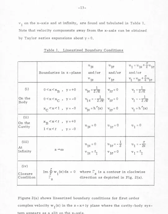
1 on the x-axis and at infinity, are found and tabulated in Table 1.

Note that velocity components away from the x-axis can be obtained

by Taylor series expansions about y = 0.

(i)

On the Body

(ii)

On the Cavity (iii) At Infinity (iv) Closure Condition

Table 1. Linearized Boundary Conditions

(J ule: ulcr ul = ulE: +Eula

Boundaries in z -plane and/or and/or and/or

O<x<xB _' y =+0

o

<x<xc

,

y = -0

xc <x< 1

,

y = -0

xB <x<i

'

y=+O

l<x<i

,

y = -0

z -+oo

Im

p

w

1 ( z) dz = 0

r

z

O'

v lE: v 10' vl = vle: + Evlcr

1

v₁cr = 0 1 vlE: = 2

rx

vl = 2 ./X

1

v₁cr = 0 1

vl E: = - 2 ./X vl = - 2 ./X

I

v

18 = h (x) v1cr = 0

I

v

1 = h (x)

u lE: = 0 _{ulcr =0} u₁=0

u₁₈ = 0 _{ulO' = -}

₂

1 _{u 1 = - 2E:} O'

v le: = oI v 10' = 0 vl

=

6I

where

r

is a contour in clockwise

z

direction as depicted in Fig. 2(a).

Figure 2(a) shows linearized boundary conditions for first order

complex velocity w

[image:21.563.7.548.36.723.2]

The most convenient way to find an analytic function w

1 (z) is to unfold the cavity-body slit onto a single line in another plane and to

reduce the problem to a Hilbert mixed-type boundary value problem.

See, e. g. , Muskhelishvili [ 12] for this type of problem in detail.

The mapping function for this purpose is

where

and

(, =

c

J-z

z-i

C=s+i11

c = /"j'"":"[

which maps the z-plane onto C-plane as follows.

a) The cavity-body slit in z-plane --+ the real axis

S

of C-plane.

b) The whole flow field in z-plane --+ the upper half of C-plane.

c) The end point of the cavity --+ the infinity in C-plane.

d) The infinity in z-plane --+ C =ic.

e) The coordinate x in z - plane --+

11/2

s

/c2+s2

11/2

s

rx

=

-/c2+s2

for

for

s>o,

11=+0

s<O, 11=-0.

(14)

( 15)

(16)

( l 7a)

( l 7b)

The boundary conditions are also mapped onto C-plane and are shown

in Fig. 2(b). Defining a new function W

1(C) as

( 18)

we analytically continue W

(19)

Introducing the notations

(20a)

WI =WI (S-iO) = vI (S, 0) - iuI (S, 0) (20b) one can write the boundary conditions as

+

-

!!"

w

I -

w

I = 2iuI (':,, 0) = 0 for -00 < s< - I (2 I a)

+

-

I

WI + WI = 2v I ( S, 0) = 2h (x( S)) for -I < s < - Sc (2 I b)

(21 c)

+

-

.

WI-WI=21u

1(s,0)=0 for sB<s<oo (2 Id)

where the relation between x and

S

in Eq. (I 7) has been used to obtain Eq. (2 Ic). The homogeneous problem corresponding to the present problem is

+

-HI -Hl = 0 for -oo< s<-I +

-H₁+HI = 0 for -I< s< - sc +

-0 _{for -sc<s< sB} HI +HI =

+

-H₁-HI=0 for sB<s<oo

By inspection the homogeneous solution can be easily found to be

considering the conditions that no singularities be allowed at the trailing edges. With the right choice of a branch cut, i.e. , -1 to SB on s-axis, one obtains the relationships

(23a)

-oo<s<-I (23 b)

which are useful in finding the particular solution. The use of those relationships and the introduction of the new function

yield the particular solution as follows: The boundary conditions for F

1 (C) now read

+

-F 1--F 1

w1

Wi

·for -oo<s<-1

for -I<s <-sc

from Eqs. (2 la) to (2 ld), using the relations (23a) and (23b).

(24a)

(24b)

(24c)

(24d)

+

-If Fl-Fl is known on an arc

r,

the analytic solution for F

ds'

.

(2 5)

Then one can write down the particular solution for W l (

s)

as

-s

w.(CL =H (C)F

(0

=

J

(s+l)(C-s )

I~

J

c 2h'(x(s'))

1 'P i 1 B

L2'1T1

1

i/(i+s'Hs -s')

- B

~]

s'-C

(26)

using Eqs. (22) and (25), where

s'

are dummy variables for integrals.

The general complementary solution has the form of

where

n=-oo

and Pl (

s)

can be determined by the following two conditions that

i) W

1 (s)C can not have stronger singularities than W 1 (s)p,

and that

ii) w

1

(z) behaves like

l//z-i

as z-£, or

w

1

(C)

behaves like

C

as

C

-+oo.

With these restrictions the only possible form for P

1 (C) is

(2 7)

(28)

where A

can be built up from Eqs. (26) and (2 7) as

ds'

s'

-

c

~+A

+ B,.1}

s'

-

c

1 ""

(2 9)

where the symbol (~!<) denotes that the Cauchy principal value is taken for the integrals if necessary, and A

1, B1 and .R. are yet unknown real constants.

In order to qetermine three unknown quatities the boundary

condition at infinity (iii) and the closure condition (iv) are used. First define the new notations by

_K_

s'

-

c

(30a)

(30b)

(30c)

(30d)

(30e)

then W

1 (C) in Eq. (29) is rewritten as

The boundary condition at infinity (C

=

ic) is applied to W

1 ( C), then W

1 (ic)

=

v 1

+

i u1

also the closure condition to W

1 ( C), then

Im fwl(z)dz

=

Imf w1(z(C))*d'

I'z

r,

=

-ReJ

w

₁

(C)*

dC

r,

(3 1)

(32)

where I'C is a corresponding contour in

C

plane to I'z in z-plane. (See

Figs. 2(a) and 2(b).) We have three equations (two from Eq. (31) and

one from: Eq. (32 )) for the unknowns, A

1, B 1 and P., therefore we can uniquely determine them as follows. Since these three equations have

turned out to be linear in A

1, B1 and

"O""

(instead of"£"), we can write

them in the matrix form as

where

0

1

2€

0

m

12

=

Re[J1(ic)}

m

22

=

Im[J1(ic)}

a

=

m

13 = Re[J2(ic)}

m

23

=

Im [J2 (ic)}

(3 3)

(34:)

cont. Nl

=

o

₁ - Re [I₀ (ic)}

Nz

=

-Im[I₀(ic)}

N3

=

- Re{

J

_{I 0 (C)}

~C

dC}

r,

Therefore the explicit expressions for A, B and CJ are

(3 5)

. (36)

(3 7)

where

(38)

Now the problem is restated: given a geometry of the hydrofoil, its upstream flow condition and the length of cavity "£" (instead of "CJ"), we have found the first order linearized solution, the outer solution, and the cavitation number "CJ". Now one can write the velocity distri

-bution q

2

+

2

u v

u2

c

body

=

1+2e:u₁1 +

oce:

2)

body

with Eqs. (21) and (3

1

), thus

qo

2

U

=

1

+

e:u ₁

+

0 (

e: )

c

body

where

u₁j =Im(W

1(s,+O)} for -l<s<sB body

(3 9)

(40)

using relation (18). One can notice that the asymptotic expansion for

the outer solution of Eq. (39) is not valid for

S

=0(€) or x=O(e:2) because

Im(W

1 (S, +O)} has l/s or l/x

112

singularities, which can be easily seen

from Eq. (29). The series expansion in

e:

then diverges for that region

(the inner region). This fact suggests that we stretch the x-y

coordi-nates in this region by the factor

e:

2, and find the local non-linear

solution of the inner solution in the inner region so obtained.

3. Inner Solution. As implied in the foregoing discussion, we stretch

the coordinate system near the leading edge by the stretching factor

e:

2

to find the inner region. Therefore the new coordinates X and Y

(called the "inner variables") are expressed by

and (41)

y =

±/X.

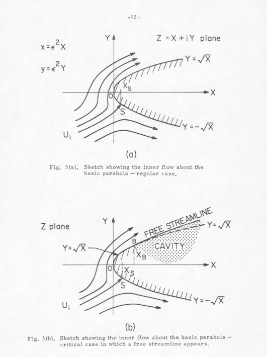
(42)

The flow configuration in the inner region (after stretching) is shown

in Fig. 3(a) or Fig. 3(b), depending on the location of the upper separa -tion point of the cavity.

Figure 3(a) shows the regular case in which the cavity separa -tion point is in the outer region, whereas Fig. 3(b) shows the critical

case in which the separation point is within the inner region.

3. 1. Regular Case. The flow around the infinitely long parabolic strut in the inner region can be constructed by the superposition of two simple

flows; the parallel uniform flow to the axis of the parabola and the

exterior corner flow turning around the parabolic nose, as schemati -cally shown in Fig. 3 (a). One can easily find the complex potential for

this flow with the help of conformal mapping function

(43)

This function transforms the flow field made by the parabolic strut

Y =

±/X

in the Z-plane onto the left half ft- plane where ft= A.+ iµ. Now

the two flows mentioned above appear in the K-plane as a local stagnation

flow perpendicular to the wall and a parallel flow along the wall. The

complex potentials which express the flows are

W - -U.ft2

s l (44a)

and

W

=

-iU x.

p p (44b)

respectively, where U. and U are the magnitudes of local uniform

l p

Superposing these two complex potentials, one obtains the complex potential W. for the inner solution as follows

l

W. _l

=

W +W _{s . p}

= -U. x.2 - iU x.

l p

(45)

where additional as yet unknown constants b and d have been introduced. The velocity profile q. on the parabolic strut is then

l

[

-2 dW. dW. ·

qi = ( dZ1 )( dZ1)

J

.

body Since

dw. 1

dZ1 body= [

dwi dx.

JI

=

dx. ·dz body -2u. (x.+ ib).

-1

-

j

i 1-21'<. body Eq. (46) becomes

2 _ ₄u2[x.+ib _ x.-ib

Jj

_

_{4 u2 x."K-ib(x.-"K)+b}2

I

qi - i 1-21'<. 1-2;{ body - i l -2(K+K)+4x.x. body

(46)

- 2 2

On the body KK = µ , K-K = 2iµ, x.+ X:

=

0, and µ

=

X due to the

transforma-tion of Eq. (43 ), q. is now written in the inner variable X as

l

2 2

q~ =

4

U~ µ +2bµ +b

l l 1+4µ2

~i.

=

j

1/4~

x

1

1

±:1n

1

.

l

x

or

or in terms of x=

e

2X, the velocity profile on the body is then

~i.

=J

2 x 11 ±

~~2

1

1 _{€ /4+x x}

(4 7)

where the upper sign is used for the upper half portion of the body, and

the lower sign for the lower half portion of the body. U. and b are as

1

yet unknown parameters which represent the magnitude of the local uniform flow speed and the location of the stagnation point respectively. These two parameters which characterize the inner flow are determined

·later by matching with the outer solution. Before proceeding to this matching procedure we first treat the critical case mentioned before.

3. 2. Critical Case. Due to the appearance of the free streamline in

the inner region there is no easy way to find the exact inner solution as for the regular case. See Fig. 3(b) for the flow configuration. Never-theless, a simple assumption on the location of the free streamline makes it possible to formulate and solve the problem with the hodograph

vari-able to a sufficient accuracy. The assumption made here is to satisfy

the boundary condition for the free streamline on the extension of the nose shape; that is, the upper body-cavity profile is also expressed by Y =

IX,

so that the same transformation used for the regular case will map the body-cavity system onto a straight line. All other boundary conditions used for the non-linear technique remain exact. This

approximate inner solution so obtained is verified later to be sufficiently

complete to permit matching with the outer solution. The final results

are then found to be accurate for the order desired. The hodograph variable

w.

is defined by

1

dW.

i9 iw.

1

U.e 1

dZ

=

q.e 1

=

1 (48)

where W. is a complex potential and U. is the magnitude of the local

uniform flow speed in Z-plane. Therefore

W. = 8

+

i T 1

The conformal mapping

Z = iK+x.2

T=fni}

1

K = A.+ iµ

(49)

(50)

maps the boundary of the parabolic body-cavity system onto the real

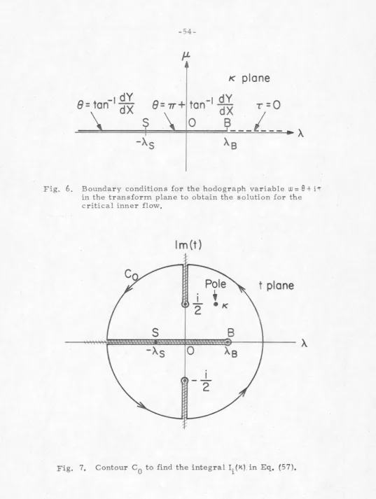
A. axis and also the flow field in the Z-plane onto the upper half K-plane. The coordinate relation between X and A. on the body is found to be

(51)

Therefore, one can write the boundary conditions in the K-plane as

T

=

0

-1 dY

90 =tan dX

-1 dY

= iT +tan dX (52)

where -A.S and A.B correspond to XS and XB' respectively. The boundary conditions in the K-plane are shown in Fig. 6. Again this problem can be reduced to a Hilbert mixed-type boundary value problem as was done

for the outer solution in Chapter 2. First the analytical continuation of

w.

(x.) into the lower half K-plane is done by

1

W. {K)

=

W. {K),

1 1

which leads one to write the boundary conditions as

+

-w

₁

.

+

w.

₁ = 2 90

+

-w. -

w.

= 0

1 1

(53)

Consider the new function F. (i-t) defined by l

where H. {X.) is the homogeneous solution to this problem which is easily l

found to be

.Jx.

-

AB by inspection. Now the boundary conditions of

Eqs. (521) for the new function F. (x.) are written as l

+

-F. -F.

l l

+

-F. -F.

l l We now observe that

and

+

-H.

=

H. l l

290

=

iv~

B

-oo<A<AB

=

0

-H~

l -oo <A< AB

( 52 II)

One can solve for

w.

(x.) by applying Plemelj' s formula to Eqs. (5211) ,

l namely,

W. (K) = H. (K)F. (X.)

l l l

(54)

The arbitrary polynomial P(K) must be zero in this case to satisfy the boundary conditions at infinity, namely, Wi

=

9

+

i T

=

0.

Substituting 9

where

ft. -1 dY

J

B tan dX dA.

lb (K)

=

---:====~ ~.

-oo /ft.B _ft.

I (K) has the closed form a

(541)

(55)

(56)

( 55 I)

The contour integral method is used to find a closed form for Ib(K) as

follows. Since

then

dY _ ± - 1 - _ 1

dX

-2

/X - 2X

-1 dY -1 1

tan dX = tan

2X

= _2i 1 _in

Define a new contour integral in the t plane, defined in Fig. 7, by

-1 1 i

r.pq

=I

tan

u

~

=

I

~£n

t

+~

._1 _ _ dt

l It-A_ t-X. 21 t-~ lt-L t-X. C

0 .. B

c

0 2 "B

(57)

where

c

0 is the contour depicted in Fig. 7. The reason why tan- 1

i

A.

is rewritten as

ii

£n (t+i/2)/(t-i/2) is that it is easier to identify the

branch points in this form. By the Cauchy integral formula

-1 1

tan -2

-

x.

I. ( x.)

=

2iri

The contour integral itself along

c

0 is a tedious but straightforward calculation and here only the result is given

I. ( K) =

1

Equating Eqs. (58) and (59), one can find

where

(

2

1)1/2

Ro=

AB+

4

-1 -1

e

₀

=

;r +tan

zx;

( 59)

( 5 6 ')

( 60)

and A.Bis found by Eq. (51) such that

\=X~

2

.

Equations (55') and (56') are now substituted into Eq. (541) to obtain

l

e

2 0 r . ;

-i R

0 + ( ~ - K) + 2R0 sin

2 . .; \ -

x.

+

2£n 1

-

_{2 .}

e

₀

R +(L-K)-2R sin-·~ 0 "B 0 2 B

( 54 ")

We are now able to express the velocity distribution on the body using the original definition for

w.

in Eq. ( 48), i. e. ,

2 2 i(U\-Wi)I

q. = U. e .

1 1

body

Since

(W.-W.)I

=

2iim[w.pq}

I

,

1 1 1

body X.-A< A

-

B

and

I

I

As+ Al

I [

w

.

(

x.) }

=

in

---;;::::::===::--:====--:----:---m i ' ' 2 JAB+ AS

,j

AB - A + 2 AB + AS - A

X.= A< f\B

we finally obtain the inner velocity distribution for the critical case

q.

1

u.

-1

(

Jxll2~

_{x1/2 +}

Jx112

_{+A )}2

B

·

B

S

8

₎₁₁₂

. CR

0

+

(x~

2

_Tx

112

₎

+

2R~

2

sin:·

j

x~

2

TXl/

2 , R ₀

+

(x1/2 _{B ~} x1;2 )- 2 R1/2 . _{O sm 2}

_g_. Jx112

_{B ~} x1/2

(61)

with the aid of Eq. (51). In terms of the outer variable x

=

e2

x

with

2

1/2

qi

'"s±TI

ui

=

(J

_XB

1/2

_{=F x}

1/2

j

_XB

1/2

)2

+ --+

t.

e:

€

s

1/2

(

1/2

::r:

1/2)

8

J

1/2

~

1/2 \.

XB T x

1/2

.

0

XB T x \

Ro+

(

1/2: 1/2

)+

2

R

0

sin~·

j

1/2;

1/2)

.

XB x

1/

2 . 0 XB x R

0 +

e:

-

2R0 sm

2 .

8 ·

(6 11)

where R

0 , 90 are given by Eq. (60). Two unknown parameters U. and l

t-5 appear in this result. These have exactly the same meaning as

those in the regular case, and they are to be determined by matching.

4. Matching. The basic notion of matching is that there exists a

common region where both the outer and inner expansions agree.

Mathematically speaking, the behavior of the outer solution as the outer

variable x tends to zero and the inner solution as the inner variable X

tends to infinity should be in agreement with each order of expansion

of the small parameter. Alternatively, the "asymptotic matching

principle" described by Van Dyke (Ref. [ 10

J,

pg. 64-68) can be applied.

In words this is

"The m-term inner expansion of (the n-term outer expansion)

=

the n-term outer expansion of (the m-term inner expansion)"

(62)

m and n may be taken as any two integers, equal or unequal. The actual

procedure following the principle of Eq. (62) is that the m-term

the inner variables; and conversely for the right-hand side of Eq. (62 ).

(In the present problem m

=

1 and n

=

2.)

In order to save time in rewriting the solutions for expansions, one can expand both inner and outer solutions in terms of the outer

variable x only. In the present case the outer solution is expanded in terms of x the order of which is 11

_e:

2 _{" (the inner region), and also the}

inner solution in terms of x the order of which is 11₁11 _{(the outer region).}

4. 1. Expansion of the Outer Solution. The two term expansion for the

outer solution is, from Eq. (39),

qo

l

U

=I+ e:ul c body

(39')

and from Eq. (40)

u i

I

=

Im { W ₁ (S ,

+

O)}

body

Now we further expand Eq. (39') for small x (note that near the nose the order of xis like

e:

2). From Eqs. (17 a, b) we obtain

x= x-+O. (63)

Therefore, as

s

-+Q(€) (64)

We now explicitly expand the velocity u

1 on the body as

Im { W

1 ( s , + O) }

I

= Im

fr

1 ( s , + O) } + Im {r2 ( s ,

+

o) } body

Each of these terms is expanded fir st in terms of

S and then in x

through Eq. (63). There are two cases to consider, the regular case and the critical case. We consider first the regular case. The first term in Eq. (401) becomes

(6 5)

=

-

;

F;

I~

(0, +O) + 0( e) (6

s')

where

-s

r'

(s, +o)

=

*f

c

h'(x(s')) .

~

1

/(i+s')(s -s') s'-s

-1 B

(66)

For the second term we have

Im [1

2 ( S, +O)}

I

= body

(6 7)

(6 7')

where

(68)

The third term is

Im[Jl(s,+o)}j

=

~(l+S)(SB-S)

body

(69)

=

JF:;;"

+

O( e)

*':<

I 2

fa(s,+O) seems to have a singularity as t;-+O(E: ), because of the l/s term in front of the bracket, but this behaves like a constant as s -+O.

and lastly the fourth term is

( 70)

vts;

r--- ( 1 )

= - s - + YSB

1--r

+0(€)

B

(70')

Therefore for the regular case the leading term required for matching with the inner solution is found in Eq. (701) , i. e. ,

where SB= 0(1 ). In terms of x this is

(71)

We now treat the critical case (xB = O(e2), SB= 0(€)). The

expansion is slightly different because "SB-s11 _{is now of the same order}

as €, so that

Again, this is rewritten in terms of x using Eq. (63) to obtain

1/4

J

1/2

+

1/2 i. XB x

= l - e:B 1

172

1/2

c x

The negative sign is used here because the matching p1·ocess is carried out on the lower half of the body.

4. 2. Expansions of the Inner Solution. As before we begin by treating the regular case. From Eq.

(47

1) ,

qi

J

x

ui

=

₈2

- + x

4

which has the two term expansion

I

1

±

~f2

I

x

qi

e:

b

u.

=

l ±

172 .

(73)

1 x

The critical case is obtained from Eq. (61 '). After the lengthy algebraic calculations one can find the expansion as

J

1/2

1/2

~ff::/2

)

qi

1/2

XB

+

x XB

u

= 1 - e: 1/2 2

-e:-

+ "-s

- so

c x

1/2 1/2

1

~x~

2

+

x

1

1

2

)

~

r;;rzz-

~

+e:z-

1/2 2

J-%--e:-++~"s-so

x (x

)

2~

~+

A.

.

+ E:

e:

E:

s

+0(€3/2) x

x

(74)

where

(75)

Note that the last term is found to be of order

e:

312, not

e:

2 as in the

regular case~

4. 3. Matching for the Regular Case. We now equate the leading terms of Eqs. ( 71 ), (73) to determine the unknown parameters U. and b.

1 They are

u.

=

u

(76b)

4. 4 Matching for the Critical Case. A similar process with Eqs. (72),

(74) allows the parameters ui and ~ to be found,

u.

=

u

1 c (77a)

XB 1/2 £1 4

~~

/2

)

·1

2

-e: -

+ A.S - S 0 =

e:

B 1 c l / 2 ' (77b)

or

(77b')

The matching has been done so that both the inner and outer solutions

behave in the same manner to the order of

e:

in some intermediate region.

We should notice, however, that the next higher order term not matched

is of order

e:

312 unlike the regular case which is matched through the

2

order of e: • But this was quite expected because of the assumption made

on the location of the free streamline. Nevertheless, the errors due to

this assumption have turned out to be as seen above of higher order.

5. Construction of Uniformly Valid Solutions. The simplest way to

construct uniformly valid solutions among others is to add the inner

and outer solutions and subtract the part they have in common. (This

both to the regular and critical cases; one can find the uniformly valid solutions as follows.

5.1. Uniformly Valid Solution for the Regular Case. Since the

common part is given by 1 ± e:b/x112 from Eq. (73), the uniformly valid solution on the body is

if-

=

j

x / 1 ±

~~

2

I

+

e:

j(

i+ s(x) )( sB - s(x))

c . e:2 / 4

+

x . x

x

[-I~

(S(1Tx), +O)

I~(s(x),

+O) ]

- 1/2 +Al

2ir f

[

~(l+s(x))(SB-s(x))

-J1sB

J

₂

+

e:Bl S(x) =f 1/2

+

O(e: ) <78 )

ex

from Eqs. (47') and (401) with (65) - (69). The upper signs are used for

the upper portion of the body and the lower signs for the lower portion of the body.

r;.

(S(x), +O) and I~(S(x), +O) are given by (66) and (68) respectively, b by (76b), A

1 and B1 by (35) and (36). Also xand Sare related through the Eqs. (l 7a) and (l 7b).

5. 2. Uniformly Valid Solution for the Critical Case. Since the common

part is

J

1/2 =f 1/2

XB

x

l /2

x

_..9._

=

u

_c

I

_{A. ± _x _ _} 1/2

I

s

€

1/2

=f X

r:;vz-)2

+J~+~

(

1/2 1/2) ₉

j

l/2 =f xl/2 RO+ xB : x +

2R~2

sin

-f ·

xB

e

1/2 1/2 1/2 1/2

(

xB =fX ) ₁₁₂ 8₀ xB =t=x R

0+ e -2R0 sin

y·

8

1/2

I

1 (S(x), +O) 12(-:o(x), +O)

[

I I J:"

J

+ e)(l+s(x))(SB-s(x)) - rr - Zrr£1/Z _{+A 1}

where I~(S(x), +O) and I~(S(x), +O) are given by (66) and (68), AS by (77b') with (60), (51) and (75), and x and Sare related by Eqs, (17 a, b). We notice that in both cases the uniformly valid solutions do not have any

singularities as x

-o.

Also notice that the solution for the critical

3/2 . 2

case has the error

e

instead of

e

for the regular case.

6. Special Cases.

6. 1. Infinite Cavity Case (.£ .... co or O'= 0) for an Arbitrary Profile Shape

·with a Parabolic Nose. For .£ .... oo, the mapping function is simplified to

s

=

±/X.

( 81)

on the real axis. Therefore

I~

( S(x), +O) / 1112 now assumes the form

from Eq. (68 ). Since

- sc

(

s'

-

s)

J (

i

+

s') (. sB

- s')

=

1

(Sc+ s)(

l+

SB)

~

( l+

s)( SB

-

S)

1.n (

J

(1-

Sc)( SB+

Sc) +

J

(1

+

S)

(SB

-

S)

)2

+ (Sc+ s

)2

(82)

and

lB

dS'

"DI (0)" -

_l_

.

en

Sc(l+sB~

-sc s' J(l+s')(sB-s'l

JsB

(~o-e:cHsB+sc)

+

lf;)

2

+

s~

(83) the uniformly valid velocity profile on the body is then for the regular case

_s.._ _

_{u -}

j

x

₁₁

± e:b

I+

e:

j(

1

±

112)( 112 112)

2

--vz

.

x XB =fX

I

~

E:B1

(Jr

_1± 1/2)( 1/2 1/2)-

1172)

O( 2) 1

± xl/2 \ x xB =f x

y

xB

+

€ )

[

I~(s(x),+0)

1 (

):f:

]

x -

·rr ± 1/2 Dl(O)-Dl(S(x).) +Al 2,,.x

(84) cont.

where

(85)

from Eq. (76b) and I~ (S(x), +O) is given by Eq. (66) and the remaining terms in the bracket are given in Eqs. (82), (83). The constants A

1, B

1 and

a

defined by Eqs. (35), (36) and (37) are reduced to simpler forms

(86)

-s

B1

=

o

-

..!..

J

c

h'(x(s')) <ls' - D1(0)

1 _{,,. - 1}

_~

_{( i+ s'}

_H

_{s - s')} 2_,,. B

(8 7)

(J

=

0 (88)

For the critical case we obtain from Eq. (79)

=fXl/2

~)

e

+

.

J++;,_s

(89)

x

1/2

1/2

j

1/2

1/2

( XB =f x )

1/2 . 90

XB =f x

R

0

+

8

+

2R

0 sin

2 .

8

1/2

xl/2 =f xl/2 .

e

R +( B

)-2R

112

sin__Q_·

0 € 0 2

1/2

.

1/2

XB =f x

€

J(

I/2)f 1/2

1/2)[

I~(s(x),+O)

t € 1 ± x \XB =f x - 'IT (89)

cont.

±

11/2

(nl(O)-Dl(S(x)))l

2'ITX

J

e:Bl

(J(i

l/2)f 1/2

1/2)

±172

± x \XB =fX

x

j

1/2

1/2)

+

0( 3/2.

- . XB =fX € )

where \, becomes

(90)

with Eqs. (51 ), (60) and (75) and B

1 remains the same.

6. 2. Parabolic Strut at Zero Cavitation Number. For the regular case as sC-+l, both

I~(s,+O),

D

1(s) go to zero, B1-+oI' and b-+o1

J:!f2.

We obtain the velocity distribution

1/4

~

J

x

I

e:oixB

I

u

=

2

l±

1/2

c e:/4+x x

±

~

1

)

2

(

J(l±xl/2)(x~2hl/2)

-Jx~z)

+

0(€2). (91)

The critical case is similarly treated to obtain

x

1/2 1/2

j

l/2 1/2

( XB =f x ) 1/2 . 9

a

XB =i= x

Ra+ e +2Ra sm-z· e

1/2 1/2

j

l/2 1/2

( XB =f x ) 1/2 . 8

a

XB =f x

Ra+

e

-

2Ra sm

_{2 ·}

e

where

2 1/2

f-s

= .!.

(e

1/2 5

+s ) -

xB

4 1

a

E.: ( 93)

6. 3. Base-Vented Parabolic Strut. This is the case in which the two detachment points are fixed at x

=

1 followed by the infinite cavity.

The velocity follows from setting xB =I in Eq. (91). We obtain

J

x

I

e

5

1

I

E.:

5

1 ( ) 2

-ff-=

2 1±172

±172

/T=X-1 +O(E:)

c E.: /4

+

x x x

(94)

This result is similar to Johnson and Rasnick' s [ 13] semi-exact ad hoc calculation for the zero angle of attack case.

7 · Numerical Results and Discussion. Theoretically the uniformly

infinite cavity was analyzed. The upper detachment points we fixed at were xB= 1.0, 0.05, 0.01, 0, and the angle of attack was set at one degree.

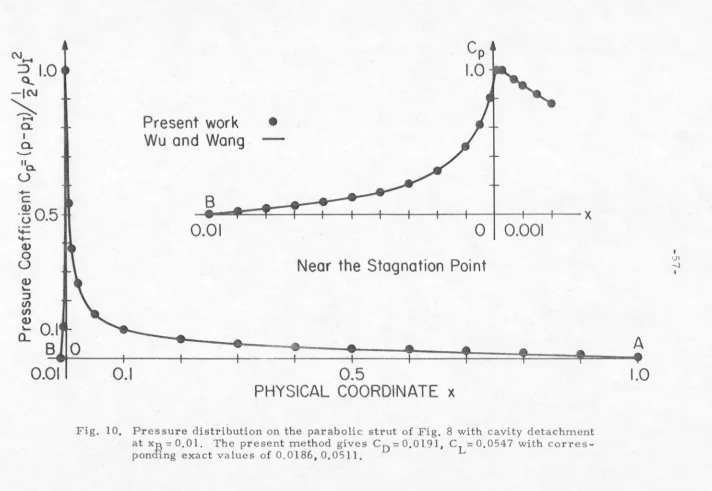
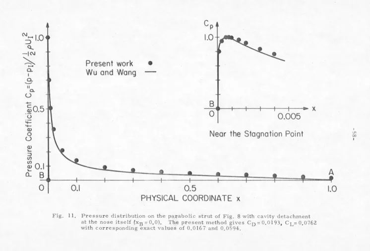
Note that the leading edge diameter, e2, is 0.01. Using the Eqs. (91), (92) and (94), we calculated the pressure distribution on these bodies. The results of these calculations are presented in Figs. 8-11 together with original calculations using Wu and Wang's exact theory [2

J.

This latter method appears to be the most direct and useful of the several exact methods now available but there are definitely numerical diffi-culties in obtaining convergent solutions. These are described more at length in Appendix B. The main point to be established here is that the present approximate method agrees very well with the exact results.

We should mention, however, differences in the two methods in the cases xB = 0.0, 0.05 (Figs. 11, 9). These errors are however of the expected order in

e

and they are not large. It should be mentioned that the matchings of the present problem have been carried out around the nose. The expansions used are not appropriate for the critical case when the cavity separation point lies in an intermediate position between the nose and the outer region. The small differences observed for the xB = 0. 05 case (Fig. 9) are due to this reason. The differences occuring for the separation at the leading edge (xB = 0, Fig. 11) are due to a

different source. In this case the upper free streamline cannot be

expected to be well approximated by the parabolic shape. As mentioned, the error in this case is of order e312 which came from the inner solution. Although the profile of the leading edge in the present method is not

linear cascade problems in Part II of this thesis), the accuracy of this

method then depends on that of the inner solution. In the case where

the simple inner flow can not be easily solved to a sufficient accuracy

for matching, or where the angle of attack and/or the cavity thickness are large, it seems more appropriate to use nonlinear exact theories

[2, 4] directly.

The pressure coefficients CL, CD calculated at the same time

also show good agreement with the exact values which are included in

the caption of each figure.

All computations were carried out on the IBM Computer 3

70-15 5 at the Booth Computing Center, California Institute of Technology.

It took about 6 to 14 minutes to obtain each convergent solution after

14 to 25 functional iterations of Wu and Wang's non-linear method,

whereas the computations by the present work took just two seconds.

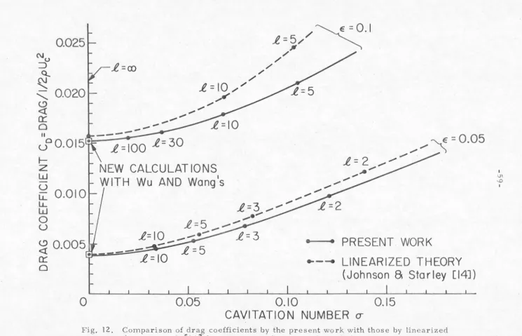
Figure 12 shows the comparison of drag coefficients computed

by the present work with those determined from the full linearized free

streamline theory [ 14] for the base-vented parabolic struts defined by

y

=

± E:

./x.

Wu and Wang's non-linear calculation showed the same

value as those of the present work as the limiting case (f-oo) both for

E': = 0.05 and 0.1. The overestimation on the drag coefficients by the

linearized theory of Ref. [ 14] is due to its poor representation of

bluntness of the foil, especially for finite cavity length. The

over-estimation of forces is characteristic of linearized free streamline

theory.

In Figs. (13) to (15) attention has been paid to the variations of

angles of attack. This type of information may possibly indicate the cavitation separation point in a real flow, but otherwise these distributions are applicable in non-cavitating ventilating flow. It is interesting to note that in Fig. 13 the zero degree angle of attack

case indicates a smooth type of separation for xB

=

0. 01. We can also observe smooth separations for long cavity lengths at two degree angle of attack (Fig. 14). For other angles of attack and for shorter

cavity lengths negative pressure coefficients are developed near the nose (Figs. 14, 15) and the change of the fixed separation point has a

strong effect (Figs. 14-16).

Figures (16) and (17) show the variations of drag and lift

coefficients for parabolic struts with the fixed separation point

xB = 0. 01 as a function of cavitation number and angle of attack.

8. Summary. The singular perturbation method has been applied

to correct the deficiencies of linearized theory of flow past cavitating

hydrofoils with rounded noses. The differences of the local pressure coefficient between the present work and an exact theory have been found to be not large even for the most "critical" case, i.e., the case in which the cavity separation point is fixed right on the nose itself. Otherwise the agreement is excellent. The procedure of the

singular perturbation method is straightforward with the aid of

linearized free streamline theories and the standard method of complex

variable analysis. Because of its simplicity, economy, and direct

REFERENCES

1. Levi-Civita, T. 1907. "Scie e leggi di resistenzia". R. C. cir

mat. Palermo, .!.:..~.' pp 1-37.

2. Wu, Y. T. and Wang, D. P. 1963. "A wake model for free-streamline flow theory, Part 2. Cavity flows past obstacles of arbitrary profile". J. Fluid Mech., ~' pp 65-93.

3. Wu, Y. T. 1956. "Note on the linear and non-linear theories for fully cavitated hydrofoil". California Institute of Technology, Rep. 21-22. Pasadena, California, U.S. A.

4. Brodetsky, S. 1922. "Discontinuous fluid motion past circular and elliptic cylinders". Proc. Royal Society of London, A 102, pp 542-553.

5. Oba, R. 1964. "Theory for supercavitating flow through an arbitrary hydrofoil". J. of Basic Eng. ASME 86, pp 285-290. 6. Larock, B. E. and Street, R. L. 1968. ''Cambered bodies in

cavitating flow - A non-linear analysis and design procedure". J. of Ship Res. 9, pp 1-13.

7. Murai, H. and Kinoe, T. 1968-1969. "Theoretical research on blunt-nosed hydrofoil in fully cavitating flow". Rep. Inst. High

Sp. Mech. 20. Tohoku, University, Sendai, Japan.

8. Tulin, M. P. 1953. "Steady two-dimensional cavity flows about slender bodies". DTMB Report 834, Navy Department,

Washington, D. C.

9. Tulin, M. P. 1964. "Supercavitating flows - Small perturbation theory". J. of Ship Res.

J_,

pp 16-37.

10. Van Dyke, M. 1964. "Perturbation methods in fluid mechanics". Academic Press.

11. Cole, J. D. 1968. "Perturbation methods in applied mathematics". Blaisdel Pub. Co.

12. Muskhelishvili, N. I. 1946. "Singular integral equations".·