R E S E A R C H
Open Access
Viscosity iterative algorithm for the zero
point of monotone mappings in Banach
spaces
Yan Tang
1**Correspondence: [email protected] 1College of Mathematics and
Statistics, Chongqing Key Laboratory of Social Economy and Applied Statistics, Chongqing Technology and Business University, Chongqing, China
Abstract
Inspired by the work of Zegeye (J. Math. Anal. Appl. 343:663–671,2008) and the recent papers of Chidume et al. (Fixed Point Theory Appl. 2016:97,2016; Br. J. Math. Comput. Sci. 18:1–14,2016), we devise a viscosity iterative algorithm without involving the resolvent operator for approximating the zero of a monotone mapping in the setting of uniformly convex Banach spaces. Under concise parameter
conditions we establish strong convergence of the proposed algorithm. Moreover, applications to constrained convex minimization problems and solution of Hammerstein integral equations are included. Finally, the performances and
computational examples and a comparison with related algorithms are presented to illustrate the efficiency and applicability of our new algorithm.
MSC: 47H04; 46N10; 47H06; 47J25
Keywords: Monotone mapping; Zero point; Viscosity approximation; Strong convergence
1 Introduction
LetHbe a real inner product space. A mapA:D(A)⊂H→2His called monotone if, for
eachx,y∈D(A), the following inequality holds:
ξ–η,x–y ≥0 for allξ∈Ax,η∈Ay. (1.1)
Interest in monotone mappings derives mainly from their significant numerous appli-cations. For example, the classical convex optimization problem: leth:H→R∪ {∞}be a proper convex, lower semicontinuous (l.s.c.) function. The sub-differential ofhatx∈H is defined by∂h:H→2H
∂h(x) =x∗∈H:h(y) –h(x)≥y–x,x∗,∀y∈H.
Clearly,∂his a monotone operator onH, and 0∈∂h(x0) if and only ifx0is a minimizer
ofh. In the case of setting∂h≡A, solving the inclusion 0∈Au, one obtains a minimizer ofh.
In addition, the inclusion 0∈AuwhenAis a monotone map from a real Hilbert space to itself also appears in several systems, in particular, evolution systems:
du
dt +Au= 0,
whereAis a monotone map. At an equilibrium state, dudt = 0, so thatAu= 0, the solution coincides with the equilibrium state of the dynamical system (see, e.g., Zarantonello [4], Minty [5], Ka˘curovskii [6], Chidume [7], Berinde [8], and others).
For solving the original problem of finding a solution of the inclusion 0∈Au, Martinet [9] introduced the well-known iteration method as follows: forn∈N,∀λn> 0,x1∈Eand
xn+1=Jλnxn,
whereJλn= (I+λnA)–1is the well-known Yosida resolvent operator,Ais a monotone
op-erator in Hilbert spaces.
This is a successful and powerful algorithm in finding a solution of the equation 0∈Au and after that, it was extended by many authors (see, e.g., Rockafellar [10], Chidume [11], Xu [12], Tang [13], Qin et al. [14]).
On the other hand, Browder [15] introduced an operatorT:H→HbyT=I–AwhereI is the identity mapping on a Hilbert spaceH. The operatorTis called pseudo-contractive and the zeros of monotone operatorA, if they exist, correspond to the fixed points ofT. Therefore the approximation of the solutions ofAu= 0 reduces to the approximation of the fixed points of a pseudo-contractive mapping.
Gradually, the notion of monotone mapping has been extended to real normed spaces. LetEbe a real normed space with dualE∗. A mapJ:E→2E∗, defined by
Jx:=x∗∈E∗:x,x∗=x ·x∗,x=x∗, (1.2)
is called the normalized duality map onE. Some properties of the normalized duality map can be obtained from Alber [16] and the references therein.
Since the normalized duality mapJis the identity mapIin Hilbert spaces, and so, under the idea of Browder [15], the approximating to solution of 0∈Auhas been extended to normed spaces by numerous authors (see, for instance, Chidume [17,18], Agarwal et al. [19], Reich [20], Diop [21], and the references therein), whereAis a monotone mapping fromEto itself.
Although the above results have better theoretical properties, such as, but not only, weak and strong convergence to a solution of the equation 0∈Au, there are still some difficulties to overcome. For instance, the generalized technique of converting the zero ofAinto the fixed point ofT in Browder [15] is not applicable since, in this case whenAis monotone, AmapsEintoE∗. In addition, the resolvent technique in Martinet [9] is not convenient to use because one has to compute the inverse of (I+λA) at each step of the iteration process.
Hence, it is only natural to ask the following question.
Motivated and inspired by the work of Martinet [9], Rockafellar [10], Zegeye [1], and Chidume et al. [2,3], as well as Ibaraki and Takahashi [22], we wish to provide an af-firmative answer to the question. Our contribution in the present work is a new viscos-ity iterative method for the solutions of the equation 0∈AJu, that is,Ju∈A–1(0), where
A:E∗→Eis a monotone operator defined on the dual of a Banach spaceEandJ:E→E∗ is the normalized duality map.
The outline of the paper is as follows. In Sect.2, we collect definitions and results which are needed for our further analysis. In Sect.3, our implicit and explicit algorithms without involving a resolvent operator are introduced and analyzed, the strong convergence to a zero of the composed mappingAJunder concise parameters conditions is obtained. In addition, the main result is applied to the convex optimization problems and the solution of Hammerstein equation. Finally, some numerical experiments and a comparison with related algorithms are given to illustrate the performances of our new algorithms.
2 Preliminaries
In the sequel, we shall need the following definitions and results.
LetEbe a uniformly convex Banach space andE∗be its dual space, let the normalized duality mapJonEbe defined as (1.2). Then the following properties of the normalized duality map hold (see, e.g., Alber [16], Cioranescu [23], Xu and Roach [24], Xu [25], Zăli-nescu [26]):
(i) Jis a monotone operator;
(ii) ifEis smooth, thenJis single-valued; (iii) ifEis reflexive, thenJis onto;
(iv) ifEis uniformly smooth, thenJis uniformly continuous on bounded subsets ofE. The spaceEis said to be smooth ifρE(τ) > 0 for allτ > 0, and the spaceEis said to be
uniformly smooth iflimτ→0+ρE(τ)
τ = 0, whereρE(τ) is defined by
ρE(τ) =sup
x+y–x–y
2 – 1;x= 1,y=τ
.
Letp> 1, the spaceE is said to bep-uniformly smooth if there exists a constantc> 0 such thatρE(τ)≤cτp,τ> 0. It is well known that everyp-uniformly smooth Banach space
is uniformly smooth. Furthermore, from Alber [16], we can get that ifE is 2-uniformly smooth, then there exists a constantL∗> 0 such that
Jx–Jy ≤L∗x–y, ∀x,y∈E.
A mappingA:D(A)⊂E→E∗is said to be monotone on a Banach spaceEif, for each x,y∈D(A), the following inequality holds:
x–y,Ax–Ay ≥0.
A mappingA:D(A)⊂E→E∗ is said to be Lipschitz continuous if there existsL> 0 such that, for eachx,y∈D(A), the following inequality holds:
A mappingf :E→Eis called contractive if there exists a constantρ∈(0, 1) such that
f(x) –f(y)≤ρx–y, ∀x,y∈E.
LetCbe a nonempty closed convex subset of a uniformly convex Banach spaceE. A Ba-nach limitμis a bounded linear functional onl∞such that
inf{xn;n∈N} ≤μ(x)≤sup{xn;n∈N}, ∀x={xn} ∈l∞,
andμ(xn) =μ(xn+1) for all{xn} ∈l∞. Suppose that{xn}is a bounded sequence inE, then
the real valued functionϕonEdefined by
ϕ(y) =μxn–y2, ∀y∈E, (2.1)
is convex and continuous, andϕ(y)→ ∞asy → ∞. IfEis reflexive, there existsz∈C such thatϕ(z) =miny∈Cϕ(y) (see, e.g., Kamimura and Takahashi [27], Tan and Xu [28]), so we can define the setCminby
Cmin= z∈C;ϕ(z) =min
y∈Cϕ(y)
. (2.2)
It is easy to verify thatCminis a nonempty, bounded, closed, and convex subset ofE. The following lemma was proved in Takahashi [29].
Lemma 2.1 Letαbe a real number,and(x0,x1, . . .)∈l∞such thatμ(xn)≤αfor all Banach
limits.Iflim supn→∞(xn+1–xn)≤0,thenlim supn→∞xn≤α.
Lemma 2.2(see, e.g., Tan and Xu [28], Osilike and Aniagbosor [30]) Let{an}be a sequence
of nonnegative real numbers satisfying the following relation:
an+1≤(1 –θn)an+σn, n≥0,
where{θn}and{σn}are real sequences such that (i) limn→∞θn= 0,
∞
n=1θn=∞; (ii) limn→∞σn
θn ≤0or
∞
n=0σn<∞.
Then the sequence{an}converges to0.
Lemma 2.3(see, e.g., Xu [12]) Let E be a real Banach space with dual E∗.Let J:E→E∗ be the normalized duality map,then for all x,y∈E,
x+y2≤ x2+ 2y,j(x+y), ∀j(x+y)∈J(x+y).
Lemma 2.4(Zegeye [1]) Let E be a uniformly convex and uniformly smooth Banach space. Assume that A:E∗→E is a maximal monotone mapping such that(AJ)–1(0)=∅.Then,
for any u∈E and t∈(0, 1),the path t→xt∈E defined by
xt=tu+ (1 –t)(I–AJ)xt, (2.3)
3 Main results
We now show the strong convergence of our implicit and explicit algorithms.
Theorem 3.1 Let E be a uniformly convex and2-uniformly smooth Banach space.Assume that A:E∗→E is an L-Lipschitz continuous monotone mapping such that(AJ)–1(0)=∅
and f :E→E is a contraction with coefficientρ∈(0, 1).Then the path t→xt∈E,defined
by
xt=tf(xt) + (1 –t)
I–ω(t)AJxt, (3.1)
converges strongly to an element z∈(AJ)–1(0)provided thatlim
t→0ω(tt) = 0.
Proof SinceEis 2-uniformly smooth, from Alber [16,31], we have thatJisL∗-Lipschitz
continuous, noticing thatAisL-Lipschitz continuous, thereforeI–AJis Lipschitz con-tinuous with constant 1 +LL∗.
First, we show thatxt is well-defined. Sincelimt→0ωt(t) = 0, for∀ε> 0, there existsδ> 0
such that, for allt∈(0,δ), the inequality|ω(tt)|<εholds.
Without loss of generality, we takeε> 0 such thatρ+εLL∗=b< 1, wherebis a positive
constant. Define an operatorTtasTtx=f(x) – (1 –t)ω(tt)AJx, for∀x,y∈E, we can get
Ttx–Tty=
f(x) – (1 –t)ω(t)
t AJx–f(y) + (1 –t) ω(t)
t AJy
=f(x) –f(y) – (1 –t)ω(t)
t (AJx–AJy)
≤f(x) –f(y)+(1 –t)ω(t) t
AJx–AJy ≤(ρ+εLL∗)x–y
=bx–y,
which means thatTtis a contraction. Therefore, by the Banach contraction principle, there
exists a unique fixed point ofTt denoted byxt. That is,xt=tf(xt) + (1 –t)(I–ω(t)AJ)xt,
soxtis well-defined.
Next we shall show thatxtis bounded aslimt→0ωt(t)= 0. Forx∗∈(AJ)–1(0), we have the
following estimation:
xt–x∗=f(x
t) –x∗– (1 –t)
ω(t) t
AJxt–AJx∗
≤f(xt) –f
x∗+fx∗–x∗+ (1 –t)ω(t)
t LL∗xt–x
∗
≤(ρ+εLL∗)xt–x∗+f
x∗–x∗,
hence,
xt–x∗≤
1 1 –bf
x∗–x∗, t∈(0,δ),
On the other hand, for arbitraryu∈E, (3.1) can be rewritten as
xt=tu+ (1 –t)(I–AJ)xt+t
f(xt) –u
+ (1 –t)1 –ω(t)AJxt,
hence,
(1 –t)1 –ω(t)AJxt=xt–tu– (1 –t)(I–AJ)xt–t
f(xt) –u
,
which means thatxt converges strongly to an elementz∈(AJ)–1(0) aslimt→0ωt(t)= 0
ac-cording to Lemma2.4. The proof is complete.
For the rest of the paper,{αn}and{ωn}are real sequences in (0, 1) satisfying the following
conditions:
(C1) limn→∞αn= 0,
∞
n=1αn=∞;limn→∞ωαnn= 0and
∞
n=0ωn<∞;
(C2) fis a piecewise function:f(x∗) =x∗ifx∗∈(AJ)–1(0); otherwisef(x∗)is a contractive function with coefficientρ.
Theorem 3.2 Let E be a uniformly convex and2-uniformly smooth Banach space. As-sume that A:E∗→E is an L-Lipschitz continuous monotone mapping such that Cmin∩ (AJ)–1(0)=∅and f :E→E is a piecewise function defined as(C2).Then,for any x
0∈E,
the sequence{xn},defined by
xn+1=αnf(xn) + (1 –αn)(I–ωnAJ)xn, (3.2)
converges strongly to an element z∈(AJ)–1(0).
Proof According to the definition off, it is obvious that ifxn∈(AJ)–1(0) then we stop the
iteration. Otherwise, we setn:=n+ 1 and return to iterative step (3.2). The proof includes three steps.
Step 1: First we prove that{xn}is bounded. Sinceαn→0 andlimn→∞ωαnn = 0 asn→ ∞,
there existsN0> 0 such thatαn≤16, ωαnn ≤
1
6LL∗,∀n>N0. We takex∗∈(AJ)
–1(0) orJx∗∈
A–1(0). Letr> 0 be sufficiently large such thatx
N0∈Br(x∗) andf(xN0)∈B6r(x∗).
We show that{xn}belongs toB:=Br(x∗) for all integersn≥N0. First, it is clear by
con-struction thatxN0∈B. Assuming now that, for an arbitraryn>N0,xn∈B, we prove that xn+1∈B.
Ifxn+1does not belong toB, then we havexn+1–x∗>r. From the recurrence (3.2) we
obtain that
xn+1–xn=αnf(xn) + (1 –αn)(I–ωnAJ)xn–xn.
Thus,
xn+1–xn=αn
f(xn) –xn
– (1 –αn)ωnAJxn. (3.3)
Therefore, from (3.3) and Lemma2.3and the fact thatxn+1–x∗=xn+1–xn+xn–x∗, xn+1–x∗2 =xn+1–xn+xn–x∗2
≤xn–x∗
2
+ 2xn+1–xn,j
xn+1–x∗
=xn–x∗
2
+ 2αn
f(xn) –xn
– (1 –αn)ωnAJxn,j
xn+1–x∗
=xn–x∗
2
+ 2αn
f(xn) –xn
– (1 –αn)ωnAJxn
+αn
xn+1–x∗
–αn
xn+1–x∗
,jxn+1–x∗
=xn–x∗
2
– 2αnxn+1–x∗ 2
+ 2αn
f(xn) –xn
– (1 –αn)ωnAJxn+αn
xn+1–x∗
,jxn+1–x∗
=xn–x∗
2
– 2αnxn+1–x∗ 2
+ 2αn
f(xn) –x∗
+αn(xn+1–xn)
– (1 –αn)ωnAJxn,j
xn+1–x∗
,
that is,
xn+1–x∗ 2
≤xn–x∗
2
– 2αnxn+1–x∗ 2
+ 2αn
f(xn) –x∗
+α2nf(xn) –xn
–αn(1 –αn)ωnAJxn– (1 –αn)ωnAJxn,j
xn+1–x∗
≤xn–x∗
2
– 2αnxn+1–x∗ 2
+ 2αn
f(xn) –x∗
+α2nf(xn) –x∗
–αn2xn–x∗
–1 –αn2ωnAJxn,j
xn+1–x∗
≤xn–x∗
2
– 2αnxn+1–x∗ 2
+ 22αnf(xn) –x∗+α2nxn–x∗
+1 –α2nωnAJxn–AJx∗xn+1–x∗.
Sincexn+1–x∗>xn–x∗andAisL-Lipschitz andJisL∗-Lipschitz continuous
re-spectively, thus we get
αnxn+1–x∗≤2αnf(xn) –x∗+α2nxn–x∗+ 2(1 –αn)ωnLL∗xn–x∗.
Furthermore,
xn+1–x∗≤2f(xn) –x∗+αnxn–x∗+ 2(1 –αn)
ωn
αn
LL∗xn–x∗
≤2∗r 6+
r 3+ 2∗
1
6LL∗LL∗r≤r.
This is contradiction. Consequently, we can get that{xn}belongs toBfor all integers
n≥N0, which implies that the sequence{xn}is bounded, so are the sequences{f(xn)}and
{AJxn}.
Moreover, it is easy to see thatxn+1–xn →0 becauseαn→0 andωn=o(αn),
xn+1–xn ≤αnf(xn) –xn+ (1 –αn)ωnAJxn →0.
Step 2: We show thatlimn→∞supz–f(xn),j(z–xn+1) ≤0, wherez∈Cmin∩(AJ)–1(0). Since the sequences{xn}and{f(xn)}are bounded, there existsR> 0 sufficiently large
such thatf(xn),xn∈B1:=BR(z),∀n∈N. Furthermore, the setB1is a bounded closed and
convex nonempty subset ofE. By the convexity ofB1, we have that (1 –t)z+tf(xn)∈B1.
Then it follows from the definition ofϕthatϕ(z)≤ϕ((1 –t)z+tf(xn)). Using Lemma2.3,
we have that
xn–z–t
f(xn) –z
2
≤ xn–z2– 2t
f(xn) –z,j
xn–z–t
f(xn) –z
thus taking Banach limit overn≥1,
μxn–z–t
f(xn) –z
2
≤μxn–z2– 2tμ
f(xn) –z,j
xn–z–t
f(xn) –z
,
which means that
2tμf(xn) –z,j
xn–z–t
f(xn) –z
≤μxn–z2–μxn–z–t
f(xn) –z
2
=ϕ(z) –ϕz+tf(xn) –z
≤0,
that is,
μf(xn) –z,j
xn–z–t
f(xn) –z
≤0.
By using the weak lower semi-continuity of the norm onE, we get the following ast→0:
f(xn) –z,j(xn–z)
–f(xn) –z,j
xn–z–t
f(xn) –z
→0.
Thus, for∀ε> 0, there existsδ> 0 such thatt∈(0,δ),n≥1
f(xn) –z,j(xn–z)
<f(xn) –z,j
xn–z–t
f(xn) –z
+ε,
therefore,
μf(xn) –z,j(xn–z)
<μf(xn) –z,j
xn–z–t
f(xn) –z
+ε.
In view of the arbitrariness ofε, we have that
μf(xn) –z,j(xn–z)
≤0.
From the norm-to-weak* uniform continuity ofJon each bounded subset ofE, we have that
lim
n→∞
f(xn) –z,j(xn+1–z)
–f(xn) –z,j(xn–z)
= 0.
Thus, the sequence{f(xn) –z,j(xn–z)}satisfies the condition of Lemma2.1, so we have
that
lim sup
n→∞
f(xn) –z,j(xn+1–z)
≤0. (3.4)
Step 3: Next we show thatxn+1–z →0.
From (3.2), (3.3) and Lemma2.3we have that
xn+1–z2 =xn+1–xn+xn–z2
=xn–z+αn
f(xn) –xn
– (1 –αn)ωnAJxn
=(1 –αn)(xn–z) +αn
f(xn) –z
– (1 –αn)ωnAJxn
2
≤(1 –αn)2xn–z2+ 2
αn
f(xn) –z
– (1 –αn)ωnAJxn,j(xn+1–z)
.
In view of the fact that the sequence{xn} is bounded, without loss of generality, we
assume thatM:=sup{xn–z}, therefore,
xn+1–z2≤(1 –αn)2xn–z2+ 2
αn
f(xn) –z
– (1 –αn)ωnAJxn,j(xn+1–z)
= (1 –αn)xn–z2+ 2
αn
f(xn) –z
,j(xn+1–z)
+ 2(1 –αn)ωnAJz–AJxnxn+1–z
≤(1 –αn)xn–z2+σn,
whereσn= 2αn(f(xn) –z),j(xn+1–z)+ 2ωnLL∗M2.
From Lemma2.2and (3.4) we shall obtain that
lim
n→∞xn–z= 0,
which means that the consequence{xn}converges strongly toz. The proof is complete.
Theorem 3.3 Let E be a uniformly convex and2-uniformly smooth Banach space.
As-sume that A:E∗→E is an L-Lipschitz continuous monotone mapping such that Cmin∩ (AJ)–1(0)=∅.Then,for any x
0∈E,the sequence{xn}defined by
xn+1=αnxn+ (1 –αn)(I–ωnAJ)xn (3.5)
converges strongly to an element z∈(AJ)–1(0).
Proof Similar to the proof in Theorem3.2, we can obtain that the sequences{xn}and
{AJxn}are bounded. Furthermore, we have thatlimn→∞supxn–z,j(xn+1–z) ≤0, where
z∈Cmin∩(AJ)–1(0).
In addition, the recurrence (3.5) can be rewritten as
xn+1=xn– (1 –αn)ωnAJxn.
It is easy to see thatxn+1–xn= (1 –αn)ωnAJxn →0 asαn→0.
From the recursion (3.5) and Lemma2.4we have that
xn+1–z2 =(1 –αn)(xn–z) +αn(xn–z) – (1 –αn)ωnAJxn
2
≤(1 –αn)2xn–z2+ 2αn
xn–z,j(xn+1–z)
– 2(1 –αn)ωn
AJxn,j(xn+1–z)
≤(1 –αn)xn–z2+ 2αn
xn–z,j(xn+1–z)
+ 2(1 –αn)ωnLL∗M2
≤(1 –αn)xn–z2+ 2αn
xn–z,j(xn+1–z)
where M:=sup{xn–z}. It follows from Lemma2.2thatlimn→∞xn–z= 0, which
means that the sequence{xn}converges strongly to an elementz∈(AJ)–1(0). The proof is
complete.
According to Zegeye [1] and Liu [32], for a mappingT:E→E∗, a pointx∗∈Eis called a J-fixed point ofTif and only ifTx∗=Jx∗andTis called semi-pseudo if and only ifA:=J–T is monotone. We can observe that a zero point ofAis theJ-fixed point of a semi-pseudo mapping. IfEis a Hilbert space, the semi-pseudo mapping and theJ-fixed point coincide with a pseudo-contractive mapping and a fixed point of pseudo-contraction, respectively. In the case that the semi-pseudo mappingTis fromE∗toE, we have thatAJ:= (J–1–T)J
is monotone and theJ-fixed point set is denoted byFJ(T) ={x∈E,x=TJx}. We have the
following corollaries for semi-pseudo mappings fromE∗toE.
Corollary 3.4 Let E be a uniformly convex and2-uniformly smooth Banach space.Assume that T:E∗→E is an L-Lipschitz continuous semi-pseudo mapping such that Cmin∩FJ(T)=
∅and f :E→E is a piecewise function defined as(C2).Then,for any x0∈E,the sequence
{xn}defined by
xn+1=αnf(xn) + (1 –αn)
(1 –ωn)I+ωnTJ
xn
converges strongly to an element z∈FJ(T).
Corollary 3.5(Zegeye [1]) Let E be a uniformly convex and2-uniformly smooth Banach space.Assume that A:E∗→E is an L-Lipschitz continuous monotone mapping such that Cmin∩(AJ)–1(0)=∅.Then,for any u∈E,the sequence xndefined by
xn+1=αnu+ (1 –αn)(I–ωnAJ)xn
converges strongly to an element z∈(AJ)–1(0).
Proof Takef(x)≡uin Theorem3.2, the result is obtained.
If we change the role ofEandE∗, then we shall obtain the following results.
Theorem 3.6 Let E be a uniformly convex and2-uniformly smooth Banach space. As-sume that A:E→E∗ is an L-Lipschitz continuous monotone mapping such that Cmin∩ (AJ–1)–1(0)=∅.Then,for any x
0∈E,the sequence{xn}defined by
xn+1=J–1
αnJxn+ (1 –αn)(J–ωnA)xn
, n≥1,
converges strongly to an element z∈(AJ–1)–1(0).
Theorem 3.7(Zegeye [1]) Let E be a uniformly convex and2-uniformly smooth Banach space.Assume that A:E→E∗is an L-Lipschitz continuous monotone mapping such that Cmin∩(AJ–1)–1(0)=∅.Then,for any u∈E,the sequence{xn}defined by
xn+1=J–1
αnJu+ (1 –αn)(J–ωnA)xn
, n≥1,
We give below two examples in order to show that the conditions of explicit iterative Algorithm (3.2) are easily satisfied.
Example1 We take the parameters as follows:
αn=
1
(n+ 1)p, ωn=
1
n(n+ 1)p, (0 <p≤1).
It is easy to verify that (1) limn→∞αn= 0,
∞
n=1αn=∞; (2) limn→∞ωαnn= 0and
∞
n=1ωn<∞.
Example2 We take the parameters as follows:
αn=
1
lnp(n+ 1), ωn=
1
nlnp(n+ 1), (0 <p≤1).
It is easy to verify that (1) limn→∞αn= 0,
∞
n=1αn=∞; (2) limn→∞ωn
αn = 0and
∞
n=1ωn<∞. 4 Applications
In this section, we consider the constrained convex minimization problems and the so-lution of Hammerstein integral equations as the applications of our main result which is proposed in Sect.3.
4.1 Application to constrained convex minimization problems
In this subsection, we will consider the following minimization problem:
min
x∈Ch(x), (4.1)
whereC is a nonempty closed convex subset ofE, andh:C→Ris a real-valued con-vex function. Assume that problem (4.1) is consistent (i.e., its solution set is nonempty). According to Diop et al. [21],x∈Eis a minimizer ofhif and only if 0∈∂h(x).
Lemma 4.1 Let E be a real normed smooth space and h:E→Rbe a differential convex function.Assume that the function h is bounded,then the sub-differential map∂h:E→R is bounded and the following inequality holds:
∂h(x) –∂h(y),x–y≥ Jx–Jy,x–y, ∀x,y∈E.
Proof Defineg:=h–12 · 2, thenh=g+1
2 · 2. Sincehand · 2are differential, sog
is differential and the sub-differential ofgis denoted by∂g=∂h–J. Letx∈E, we can get from the definition of∂gthat
which means that
h(y) –1 2y
2–h(x) +1
2x
2≥y–x,∂h(x) –Jx, ∀y∈E. (4.2)
Exchangingxandyin the above inequality (4.2), we have that
h(x) –1 2x
2–h(y) +1
2y
2≥x–y,∂h(y) –Jy, ∀x∈E. (4.3)
Adding the above inequalities (4.2) and (4.3), we get that
∂h(x) –∂h(y),x–y≥ x–y,Jx–Jy.
This completes the proof.
Remark4.2 From Lemma4.1, the sub-differential∂his monotone, we can also get that T=J–∂his a semi-pseudo mapping fromEtoE∗.
Consequently, the following theorems are obtained.
Theorem 4.3 Let E be a uniformly convex and2-uniformly smooth real Banach space. Assume that h:E→Ris a proper,convex,bounded,and coercive function such that Cmin∩ (∂hJ)–1(0)=∅and f :E→E is a piecewise function defined as(C2).Then,for any x0∈E,
the sequence{xn}defined by
xn+1=αnf(xn) + (1 –αn)(I–ωn∂hJ)xn, n≥1,
converges strongly to an element x∗∈(∂hJ)–1(0),that is,Jx∗∈(∂h)–1(0).Then function h
has a unique minimizer Jx∗∈E∗and the sequence{xn}.
Theorem 4.4 Let E be a uniformly convex and2-uniformly smooth real Banach space. Assume that h:E→Ris a proper,convex,bounded,and coercive function such that Cmin∩ (∂hJ)–1(0)=∅.Then,for any x
0∈E,the sequence{xn}defined by
xn+1=αnxn+ (1 –αn)(I–ωn∂hJ), n≥1,
converges strongly to an element x∗∈(∂hJ)–1(0),that is,Jx∗∈(∂h)–1(0).
4.2 Application to solution of Hammerstein integral equations
An integral equation (generally nonlinear) of Hammerstein type has the form
u(x) +
k(x,y)fy,u(y)=w(x), (4.4)
where the unknown functionuand the inhomogeneous functionwlie in a Banach space Eof measurable real-valued functions.
By simple transformation, (4.4) shall be written as
which can be illustrated, without loss of generality, as
u+KFu= 0. (4.5)
For the case of a real Hilbert space H, forF,K:H→H, Chidume and Zegeye [33] defined an auxiliary map on the Cartesian productE:=H×H,T:E→Eby
T[u,v] = [Fu–v,Kv+u].
It is known that
T[u,v] = 0 ⇔ uis the solution of (4.5) andv=Fu.
They obtained strong convergence of an iterative algorithm defined in the Cartesian prod-uct spaceEto a solution of Hammerstein Eq. (4.5).
In a Banach space more general than a Hilbert space, Zegeye [34], Chidume and Idu [35] introduced the operatorT:E×E∗→E∗×E:
T[u,v] = [Ju–Fu+v,J∗v–Kv–u],
whereF:E→E∗andK:E∗→Eare monotone mappings andJ∗is the normalized
du-ality map from E∗ to E. They proved that the mappingA:=J–T defined byA[u,v] := [Fu–v,Kv+u] is monotone andu∗ is a solution (when they exist) of the Hammerstein equationu+KFu= 0 if and only if (u∗,v∗) is a zero point ofA, wherev∗=Fu∗. Applying our Theorem3.2, the following theorems shall be obtained.
Theorem 4.5 Let E be a uniformly convex and2-uniformly smooth Banach space. As-sume that F:E→E∗,K:E∗→E are Lipschitz continuous monotone mappings such that Hammerstein Eq. (4.5)is solvable and f1:E→E,f2:E∗→E∗are two piecewise functions
defined as(C2).Then,for(u0,v0)∈E×E∗,the sequences{un}and{vn}defined by
un+1=αnf1(un) + (1 –αn)
un–ωnJ∗(Fun–vn)
,
vn+1=αnf2(vn) + (1 –αn)
vn–ωnJ(Kvn+un)
,
converge strongly to u∗and v∗,respectively,where u∗is a solution of u+KFu= 0with v∗= Fu∗.
Theorem 4.6 Let E be a uniformly convex and2-uniformly smooth Banach space. As-sume that F:E→E∗,K:E∗→E are Lipschitz continuous monotone mappings such that Hammerstein Eq. (4.5)is solvable.Then,for(u0,v0)∈E×E∗,the sequences{un}and{vn},
defined by
un+1=αnun+ (1 –αn)
un–ωnJ∗(Fun–vn)
,
vn+1=αnvn+ (1 –αn)
vn–ωnJ(Kvn+un)
,
5 Numerical example
In the sequel, we give a numerical example to illustrate the applicability, effectiveness, efficiency, and stability of our viscosity iterative algorithm (VIA). We have written all the codes in Matlab R2016b and they are preformed on a LG dual core personal computer.
5.1 Numerical behavior of VIA
Example LetE=R,C=E. LetA,J:R→Rbe the mappings defined as
Ax=ax, Jx=x,
f:C→Cbe defined as
f(x) = ⎧ ⎨ ⎩ x
2, Ax= 0,
x, ifAx= 0.
Thus, forx,y∈R, we have
Ax–Ay=ax–ay ≤ |a| ∗ x–y,
Jx–Jy=x–y.
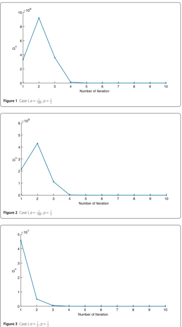
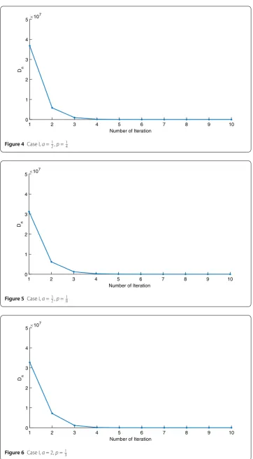
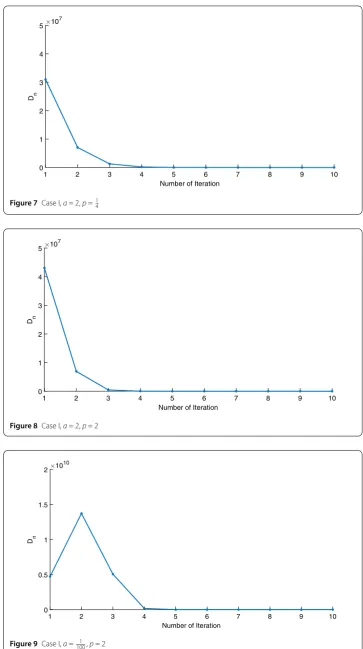
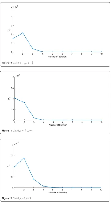
Hence,Ais|a|-Lipschitz continuous monotone,Jis 1-Lipschitz continuous. Two groups of consequences of parameters are tested here as follows: Case I:αn=(n+1)1 p,ωn=n(n1+1)p,p∈[1/8, 1/4, 1/3, 1/2, 1];
Case II:αn=lnp(1n+1),ωn=nlnp1(n+1),p∈[1/8, 1/4, 1/3, 1/2, 1].
We can see that all these parameters satisfy the conditions: (i) limn→∞αn= 0,
∞
n=1αn=∞; (ii) ωn=o(αn),
∞
n=1ωn<∞.
We will use the sequenceDn= 108×xn+1–xn2to study the convergence of our explicit
viscosity iterative algorithm (VIA). The convergence ofDnto 0 implies that the sequence
{xn}converges tox∗∈(AJ)–1(0). To illustrate the behavior of the algorithm, we have
per-formed experiments for both number of iterations (iter.) and elapsed execution time (CPU time—in the second). Figures1–18and Table1describe the behavior ofDngenerated by
VIA for the aforementioned groups of parameters. It is obvious that ifxn∈(AJ)–1(0), then
the process stops andxnis the solution of problem 0∈AJu; otherwise, we shall compute
the following viscosity algorithm:
xn+1=
αnxn
2 + (1 –αn)(xn–aωnxn),
whereais different choices from [1001 ,12, 2].
In these figures,x-axes represent the number of iterations whiley-axes represent the value ofDn. We can summarize the following observations from these figures:
Figure 1Case I,a=1001 ,p=12
Figure 2Case I,a=1001 ,p=13
Figure 4Case I,a=12,p=14
[image:16.595.117.480.74.731.2]Figure 5Case I,a=12,p=18
Figure 7Case I,a= 2,p=14
[image:17.595.114.478.77.727.2]Figure 8Case I,a= 2,p= 2
Figure 10 Case I,a=1001 ,p=14
[image:18.595.117.480.75.748.2]Figure 11 Case II,a=1001 ,p=13
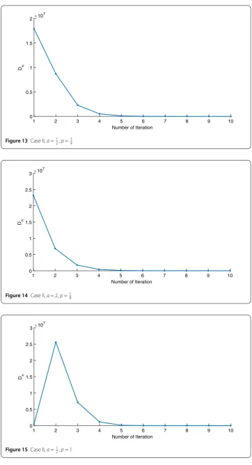
Figure 13 Case II,a=12,p=14
[image:19.595.116.479.75.744.2]Figure 14 Case II,a= 2,p=1 8
Figure 16 Case II,a=1001 ,p=12
[image:20.595.115.481.76.745.2]Figure 17 Case II,a= 2,p=13
Table 1 Algorithm (VIA) with different group of parameters
a 0.01 0.5 0.99
p= 1
Case I No. Iterations 10 10 12 CPU (time) 0.047 0.047 0.055 Case II No. Iterations 10 10 12
CPU (time) 0.044 0.048 0.045
p= 2
Case I No. of Iterations 10 10 12 CPU (time) 0.056 0.058 0.062 Case II No. Iterations 10 10 12
CPU (time) 0.068 0.055 0.052
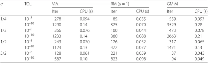
Table 2 Comparison between VIA and other algorithms withx0= 1
a TOL VIA RM (u= 1) GMIM
Iter CPU (s) Iter CPU (s) Iter CPU (s) 1/4 10–8 278 0.094 85 0.055 559 0.097
10–10 1290 0.14 325 0.070 3529 0.28
1/3 10–8 266 0.076 100 0.044 473 0.078
10–10 1233 0.14 380 0.088 2663 0.21
1/2 10–8 243 0.070 126 0.052 317 0.065
10–10 1123 0.13 472 0.077 1471 0.13
3/2 10–8 128 0.061 221 0.059 37 0.043
10–10 587 0.10 823 0.098 94 0.049
(b) Our viscosity iterative algorithm (VIA) works well for parameter sequences of{αn} being fast convergent to0asn→ ∞. In general, ifDn=xn+1–xn2, then the error ofDncan be obtained approximately equal to10–16. WhenDnobtains to this error, then it becomes unstable. The best error ofDncan be obtained approximately equal to10–30whena= 2.
(c) For the second group parameter{αn}being slowly convergent to 0 asn→ ∞, then
Dnis slightly increasing in the early iterations, and after that, it is seen to be almost stable.
5.2 Comparison of VIA with other algorithms
In this part, we present several experiments in comparison with other algorithms. Two methods used in comparison are the generalized Mann iteration method (GMIM) (Chidume et al. [35], Algorithm 1) and the regularization method (RM) (Zegeye [1], Algorithm 2). The RM requires to previously know a constant u. For experiments, we choose the same sequencesαn=n1+1 andωn=n(n1+1) in these algorithms. The condition
xn+1–xn2≤TOLis chosen to be as the stopping criterion. The following tables are
comparisons of VIA, RM, GMIM with different choices ofa. The numerical results are showed in Table2.
From these tables, we can see that the RM is the best. The GMIM is the most time-consuming, and the reasonable explanation is the fact that at each step the GMIM has no contractive parameters (coefficients) for obtaining the next step which can take lower convergence rate, while the convergence rate of the RM depends strictly on the previous constantuand the initial valuex0. In comparing with other two methods, VIA seems
[image:21.595.117.478.253.363.2]iterative algorithm works more stable than other methods and it is done in Banach spaces much more general than Hilbert spaces.
6 Conclusion
Let E be a nonempty closed uniformly convex and 2-uniformly smooth Banach space with dualE∗. We construct some implicit and explicit algorithms for solving the equation 0∈AJuin the Banach spaceE, whereA:E∗→Eis a monotone mapping andJ:E→E∗is the normalized duality map which plays an indispensable role in this research paper. The advantages of the algorithm are that the resolvent operator is not involved, which makes the iteration simple for computation; moreover, the zero point problem of monotone map-pings is extended from Hilbert spaces to Banach spaces. The proposed algorithms con-verge strongly to a zero of the composed mappingAJunder concise parameter conditions. In addition, the main result is applied to approximate the minimizer of a proper convex function and the solution of Hammerstein integral equations. To some extent, our results extend and unify some results considered in Xu [12], Zegeye [1], Chidume and Idu [2], Chidume [3,35], and Ibarakia and Takahashi [22].
Acknowledgements
The author expresses their deep gratitude to the referee and the editor for his/her valuable comments and suggestions which helped tremendously in improving the quality of this paper and made it suitable for publication.
Funding
This article is funded by the National Science Foundation of China (11471059), the Science and Technology Research Project of Chongqing Municipal Education Commission (KJ1706154), and the Research Project of Chongqing Technology and Business University (KFJJ2017069).
Competing interests
The author declares that they have no competing interests. Authors’ contributions
The author worked jointly in drafting and approving the final manuscript. The author read and approved the final manuscript.
Publisher’s Note
Springer Nature remains neutral with regard to jurisdictional claims in published maps and institutional affiliations. Received: 6 February 2018 Accepted: 9 September 2018
References
1. Zegeye, H.: Strong convergence theorems for maximal monotone mappings in Banach spaces. J. Math. Anal. Appl. 343, 663–671 (2008)
2. Chidume, C.E., Kennedy, O.I.: Approximation of zeros of bounded maximal monotone mappings, solutions of Hammerstein integral equations and convex minimization problem. Fixed Point Theory Appl.2016, 97 (2016) 3. Chidume, C.E., Romanus, O.M., Nnyaba, U.V.: A new iterative algorithm for zeros of generalized Phi-strongly
monotone and bounded maps with application. Br. J. Math. Comput. Sci.18(1), 1–14 (2016)
4. Zarantonello, E.H.: Solving functional equations by contractive averaging. Tech. Rep. 160, US. Army Math, Madison, Wisconsin (1960)
5. Minty, G.J.: Monotone (nonlinear) operators in Hilbert spaces. Duke Math. J.29(4), 341–346 (1962) 6. Ka˘curovskii, R.I.: On monotone operators and convex functionals. Usp. Mat. Nauk15(4), 213–215 (1960)
7. Chidume, C.E.: An approximation method for monotone Lipschitz operators in Hilbert spaces. J. Aust. Math. Soc. Ser. A41, 59–63 (1986)
8. Berinde, V.: Iterative Approximation of Fixed Points. Lecture Notes in Mathematics. Springer, London (2007) 9. Martinet, B.: Regularisation d’inequations variationnelles par approximations successives. Rev. Fr. Inform. Rech. Oper.
4, 154–158 (1970)
10. Rockafellar, R.T.: Monotone operators and the proximal point algorithm. SIAM J. Control Optim.14, 877–898 (1976) 11. Chidume, C.E.: An approximation method for monotone Lipschitzian operators in Hilbert-spaces. J. Aust. Math. Soc.
Ser. A41, 59–63 (1986)
12. Xu, H.K.: A regularization method for the proximal point algorithm. J. Glob. Optim.36, 115–125 (2006) 13. Tang, Y.: Strong convergence of viscosity approximation methods for the fixed-point of pseudo-contractive and
14. Qin, X.L., Kang, S.M., Cho, Y.J.: Approximating zeros of monotone operators by proximal point algorithms. J. Glob. Optim.46, Article ID 75 (2010)
15. Browder, F.E.: Nonlinear mappings of nonexpansive and accretive-type in Banach spaces. Bull. Am. Math. Soc.73, 875–882 (1967)
16. Alber, Y.: Metric and generalized projection operators in Banach spaces: properties and applications. In: Kartsatos, A.G. (ed.) Theory and Applications of Nonlinear Operators of Accrective and Monotone Type, pp. 15–50. Dekker, New York (1996)
17. Chidume, C.E.: Geometric Properties of Banach Spaces and Nonlinear Iterations. Lectures Notes in Mathematics. Springer, London (2009)
18. Chidume, C.E.: Iterative approximation of fixed points of Lipschitzian strictly pseudo-contractive mappings. Proc. Am. Math. Soc.99(2), 283–288 (1987)
19. Agarwal, R.P., Meehan, M., O’Regan, D.: Fixed Point Theory and Applications. Cambridge Tracts in Mathematics, vol. 141. Cambridge University Press, Cambridge (2001)
20. Reich, S.: A weak convergence theorem for alternating methods with Bergman distance. In: Kartsatos, A.G. (ed.) Theory and Applications of Nonlinear Operators of Accrective and Monotone Type. Lecture Notes in Pure and Appl. Math., vol. 178, pp. 313–318. Dekker, New York (1996)
21. Diop, C., Sow, T.M.M., Djitte, N., Chidume, C.E.: Constructive techniques for zeros of monotone mappings in certain Banach space. SpringerPlus4, 383 (2015)
22. Ibaraki, T., Takahashi, W.: A new projection and convergence theorems for the projections in Banach spaces. J. Approx. Theory149(1), 1–14 (2007)
23. Cioranescu, I.: Geometry of Banach Spaces, Duality Mappings and Nonlinear Problems. Kluwer Academic, Dordrecht (1990)
24. Xu, Z.B., Roach, G.F.: Characteristic inequalities of uniformly convex and uniformly smooth Banach spaces. J. Math. Anal. Appl.157, 189–210 (1991)
25. Xu, H.K.: Inequalities in Banach spaces with applications. Nonlinear Anal.16(12), 1127–1138 (1991) 26. Z˘alinescu, C.: On uniformly convex functions. J. Math. Anal. Appl.95, 344–374 (1983)
27. Kamimura, S., Takahashi, W.: Strong convergence of a proximal-type algorithm in Banach spaces. SIAM J. Optim.13(3), 938–945 (2002)
28. Tan, K.K., Xu, H.K.: Approximating fixed points of nonexpansive mappings by Ishikawa iteration process. J. Math. Anal. Appl.178(2), 301–308 (1993)
29. Takahashi, W.: Nonlinear Functional Analysis-Fixed Point Theory and Its Applications. Yokohama Publishers, Yokohama (2000)
30. Osilike, M.O., Aniagbosor, S.C.: Weak and strong convergence theorems for fixed points of asymptotically nonexpansive mapping. Math. Comput. Model.32(10), 1181–1191 (2000)
31. Alber, Y., Ryazantseva, I.: Nonlinear Ill Posed Problems of Monotone Type. Springer, London (2006)
32. Liu, B.: Fixed point of strong duality pseudocontractive mappings and applications. Abstr. Appl. Anal.2012, Article ID 623625 (2012).https://doi.org/10.1155/2012/623625
33. Chidume, C.E., Zegeye, H.: Approximation of solutions of nonlinear equations of monotone and Hammerstein-type. Appl. Anal.82(8), 747–758 (2003)
34. Zegeye, H.: Iterative solution of nonlinear equations of Hammerstein type. J. Inequal. Pure Appl. Math.4(5), Article ID 92 (2003)
35. Chidume, C.E., Idu, K.O.: Approximation of zeros of bounded maximal monotone mappings, solutions of Hammerstein integral equations and convex minimization problems. Fixed Point Theory Appl.2016, 97 (2016).