www.hydrol-earth-syst-sci.net/20/4375/2016/ doi:10.5194/hess-20-4375-2016
© Author(s) 2016. CC Attribution 3.0 License.
Combined assimilation of streamflow and snow water equivalent for
mid-term ensemble streamflow forecasts in snow-dominated regions
Jean M. Bergeron, Mélanie Trudel, and Robert Leconte
Department of civil engineering, Université de Sherbrooke, Sherbrooke, J1K 2R1, Canada
Correspondence to:Jean M. Bergeron ([email protected])
Received: 15 April 2016 – Published in Hydrol. Earth Syst. Sci. Discuss.: 26 April 2016 Revised: 29 September 2016 – Accepted: 8 October 2016 – Published: 28 October 2016
Abstract. The potential of data assimilation for hydrologic predictions has been demonstrated in many research stud-ies. Watersheds over which multiple observation types are available can potentially further benefit from data assimila-tion by having multiple updated states from which hydro-logic predictions can be generated. However, the magnitude and time span of the impact of the assimilation of an observa-tion varies according not only to its type, but also to the vari-ables included in the state vector. This study examines the impact of multivariate synthetic data assimilation using the ensemble Kalman filter (EnKF) into the spatially distributed hydrologic model CEQUEAU for the mountainous Nechako River located in British Columbia, Canada. Synthetic data include daily snow cover area (SCA), daily measurements of snow water equivalent (SWE) at three different locations and daily streamflow data at the watershed outlet. Results show a large variability of the continuous rank probability skill score over a wide range of prediction horizons (days to weeks) depending on the state vector configuration and the type of observations assimilated. Overall, the variables most closely linearly linked to the observations are the ones worth considering adding to the state vector due to the limita-tions imposed by the EnKF. The performance of the assimila-tion of basin-wide SCA, which does not have a decent proxy among potential state variables, does not surpass the open loop for any of the simulated variables. However, the as-similation of streamflow offers major improvements steadily throughout the year, but mainly over the short-term (up to 5 days) forecast horizons, while the impact of the assimila-tion of SWE gains more importance during the snowmelt pe-riod over the mid-term (up to 50 days) forecast horizon com-pared with open loop. The combined assimilation of stream-flow and SWE performs better than their individual
counter-parts, offering improvements over all forecast horizons con-sidered and throughout the whole year, including the critical period of snowmelt. This highlights the potential benefit of using multivariate data assimilation for streamflow predic-tions in snow-dominated regions.
1 Introduction
Water resource management for reservoirs located in snow-dominated regions relies on an accurate portrayal of the snow water equivalent (SWE) spatial and temporal distribution in order to make accurate streamflow predictions. Some wa-ter resources managers make use of ensemble streamflow prediction (ESP) to plan reservoir operations over various lengths of time. ESPs have the benefit of integrating weather forecast uncertainty, either by making use of weather ensem-ble predictions (de Roo et al., 2003) or by using historical weather data (Day, 1985) as input in a hydrologic model. However, ESPs depend heavily on the model’s initial con-ditions (Franz et al., 2008). Presently, many water resources managers still use a manual approach to adjust the initial state of the watershed based on available observations and the user’s experience (Liu et al., 2012).
studies have also integrated DA in ensemble forecast systems for relatively short-term (up to 5–10 days) hydrologic fore-casts (Abaza et al., 2014, 2015; He et al., 2012), but studies focusing on longer forecast periods are scarce even though the need exists for water resource managers.
Multivariate DA applications in hydrology are becoming more frequent, but generally focus on streamflow and soil moisture (Samuel et al., 2014; Trudel et al., 2014; Lee et al., 2011), omitting the snow water equivalent. In snow-dominated watersheds, the key initial states include not only information about the hydric state, such as soil moisture and streamflow, but also the snow cover state, such as SWE and snow cover area (SCA). To the authors’ knowledge, no pub-lished studies pertain to the combined assimilation of infor-mation about a watershed’s hydric and snow state. Since the lasting impact of hydric DA and snow DA can be quite dif-ferent given the difdif-ferent physical processes driving them, the simultaneous DA of both types of data could yield improve-ments over a potentially longer length of time.
However, data assimilation performance depends on vari-ous factors, such as the choice of variables to be updated by an observation (hereby referred to as the state vector config-uration). Abaza et al. (2015) demonstrated this importance when assimilating streamflow in a hydrologic model. Going from univariate to multivariate DA increases the number of degrees of freedom, which increases the complexity of the matter. The importance of state vector configuration when using multivariate DA for hydrological modelling has yet to be investigated.
The study’s main objectives are to (1) investigate the po-tential impact that multivariate data assimilation of hydric (streamflow) and snow-related (SWE and SCA) data can have on short-term (1–5 days) and mid-term (up to 50 days) streamflow forecast, and (2) to explore how this impact varies as a function of the state vector configuration.
2 Materials and methods
2.1 Study area description and data
Simulations were conducted in a synthetic setting based on the Nechako watershed located in British Columbia, Canada (Fig. 1). The watershed includes a reservoir, which drains an area of approximately 14 000 km2. The reservoir is man-aged by Rio Tinto mainly for hydroelectricity production purposes. The watershed includes part of the Coast Moun-tains in the west region, such that the difference in eleva-tion between the highest and lowest point in the watershed reaches about 1700 m. At this latitude and altitude, most (es-timated at 53 %) of the precipitation falls as snow.
There are various types of data gathered regularly over the watershed. First are the seven weather stations managed by Rio Tinto, three of which measure daily precipitation and air temperature only (yellow circles). Three others also
in-Figure 1.The Nechako watershed and the locations of weather sta-tions, snow pillows and a hydrometric station. All of these contain at least daily weather data. The outlet is considered to be at the spill-way, located at the blue triangle. The intake is located at the Tahtsa Intake weather station (westernmost yellow circle).
clude snow pillows (red squares), which measure the snow water equivalent. The northernmost snow pillow is located at Mount Wells, the southernmost at Mount Pondosy and the westernmost at Tahtsa Lake. Maximum seasonal SWE observations average 615, 853 and 1393 mm for the Mount Wells, Mount Pondosy and Tahtsa Lake snow pillows re-spectively. The distribution of snow on the ground follows a strong east–west gradient such that measurements at Tahtsa Lake typically yield much more snow than Mount Well and Mount Pondosy. The northernmost weather station (blue tri-angle) is located next to the spillway at Skins Lake and also takes hydrometric measurements. Historical daily water lev-els can then be converted into natural inflows by also taking into account spilled and turbined flow. Finally, daily SCA data derived from the spaceborne sensor MODIS/Terra are also considered (Hall et al., 2002). Because of its spatial coverage and relatively high temporal resolution, remotely sensed snow data from MODIS have proven to be valuable in a number of hydrologic studies (Bergeron et al., 2014; Roy et al., 2010; Tang and Lettenmaier, 2010; Andreadis and Let-tenmaier, 2006; Clark et al., 2006), including one applied to the Nechako watershed (Marcil et al., 2016).
[image:2.612.349.505.66.203.2]cre-Transfer function Precipitation
Snow
Forest Open area
Snowmelt Snowmelt
Available water
Ev
ap
ot
ran
sp
ir
at
ion
Ev
ap
or
at
ion
Ev
ap
ot
ran
sp
ir
at
ion
Groundwater Soil moisture Lakes
LWL HMAR
HINT HSOL SML
HINF
HNAP GWL TRI
CVSI
CVSB
CVNH
Runoff over impervious surfaces
Surface runoff
Interflow (1st)
Interflow (2nd)
“Fast” baseflow
“Slow” baseflow Rain
CVNB
In
filt
ra
ti
on
CVMAR
[image:3.612.49.283.65.409.2]CIN
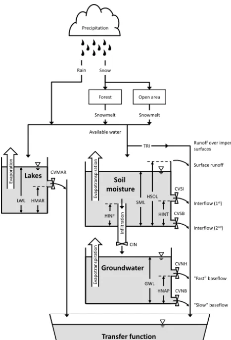
Figure 2.Diagram of the processes included in CEQUEAU’s pro-duction function.
ation of synthetic observations and meteorological input in Sect. 3.1.1 and 3.1.2 respectively.
2.2 Model description
The hydrologic model used was the spatially distributed, con-ceptual model CEQUEAU (Charbonneau et al., 1977). It is currently being used by Rio Tinto to model hydrologic pro-cesses including streamflow at the outlet of the Nechako wa-tershed, considered to be the spillway where the hydromet-ric station is also located. All variables are computed at a daily time step using a set of parameters to calibrate and daily meteorological input consisting of mean air temperature and precipitation. The set of parameters used in this study was the result of a manual calibration performed by Rio Tinto by comparing the simulated streamflow at the outlet with the corresponding real streamflow observations. A summary of the main processes concerning the production and transfer functions is presented here to facilitate the understanding of the state variables used in this study.
CEQUEAU divides the watershed into regular square pix-els called “whole squares” over which the production
func-tion is computed (Fig. 2). The current version of CEQUEAU uses the snow model presented by the US Army Corps of En-gineers (1956) to simulate most snow-related processes. The SWE is actually computed separately for forested and open areas, which have their own set of parameters, but is aggre-gated here as a weighted sum according to the proportion of forested and open areas within each whole squares. The only variable computed separately (i.e. outside from CEQUEAU) is SCA, which is computed using a depletion curve (Ander-son, 1973). The depletion curve used here follows Andreadis and Lettenmaier (2006), which uses a three parameter beta distribution:
SCAi=B−1
SWEi
min SWEmax, i,SI
|αSCA, βSCA !
, (1)
where SCAi is the resulting snow cover area over a whole
squarei, SWEi is the simulated snow water equivalent over
the same area, SWEmax, i is the annual maximum snow
wa-ter equivalent from the beginning of the accumulation pe-riod over the same area, SI represents the value of SWE above which it is assumed there is always 100 % snow cover andαSCAandβSCAare shape parameters for the beta
distri-bution itself. The calibration of those three parameters was conducted using the SCE-UA method (Duan et al., 1992) to minimize the root mean square difference between simulated snow cover area and MODIS/Terra daily L3 snow cover data (Hall et al., 2002) averaged within each whole square within the Nechako watershed. It is important to note that SCA is computed as an output only and is therefore not considered to be a state variable since it has no impact on future simula-tions if its value is tampered with.
CEQUEAU then uses three conceptual reservoirs to sim-ulate various hydrologic processes from the available water resulting from rain or snowmelt. There is an optional lake reservoir, an upper reservoir (called “soil moisture reservoir” in this study) and a lower reservoir (called “groundwater reservoir” in this study).
All in all, the state variables simulated over each whole square include SWE, a snow ripening index (SRI), a snow temperature index (STI), the soil moisture level (SML), the groundwater level (GWL) and the lake water level (LWL) should there be one. There are 644 whole squares in the case of the Nechako watershed.
follows:
SFj=
1
1t Mj X
k
extk·VOLk, (2)
where SFj is the streamflow at partial squarej,Mj is the
number of partial squares directly upstream, extkis a transfer
coefficient and1t is the time step. VOL is therefore a state variable, but streamflow, like SCA, is not considered to be a state variable since it has no impact on future simulations if its value is tampered with.
2.3 Ensemble Kalman filtering
The EnKF is a data assimilation method developed by Evensen (1994). It is an approach often used in hydrology, mainly due to its ability to consider non-linearities in the model and its relative simplicity to implement. The EnKF is a sequential method, meaning it relies only on current observa-tions to update state variables as opposed to non-sequential approaches such as smoothers (Evensen and van Leeuwen, 2000) and recursive methods (McMillan et al., 2013).
The EnKF propagates an ensemble of model runs based on a Monte Carlo implementation to represent model errors. The model covariance matrix (Pbt) at a timet is computed from the state vector (xbt) holding theN ensemble members and their simulated variables; and the ensemble mean of the state vector (xbt) therefore implicitly taking the model dynamics into consideration:
Pbt = 1
N−1 x
b t −xbt
xbt −xbt>, (3)
when an observation is available, it is perturbed to form an ensemble of observations that are used to update each ensem-ble member. The updating step applies the Kalman gain (Kt),
which is computed from observation (Rt) and model
covari-ance matrices as well as an observation operator (Ht), which
relates the model states to the observation: Kt=PbtH
> t HtPbtH
>
t +Rt
−1
, (4)
The Kalman gain acts as a weighted average between the ob-servation and state vector to yield a post-filter analysis (xat) computed as such:
xat =xbt+Kt yt−Htxtb
. (5)
The EnKF has practical and theoretical limitations. First, the EnKF relies on an ensemble representation of model and ob-servation errors that are valid in the limit where ensemble sizes approach infinity. This is not feasible in practice, so a finite sample is used instead which aims to be sufficiently large such that sampling errors are negligible while ensuring that computational power and memory limitations are met. The method also makes use of model and observation covari-ance matrices to compute the gain during the updating pro-cess. These covariance matrices assume a linear relationship
CEQUEAU
CEQUEAU Perturbation
Perturbation
Data assimilation Start
True meteorological input
3) Synthetic meteorological input
6) Hydrologic ensemble
1) True state
2) Synthetic observations
7) Analysis Ensemble perturbation
Ensemble perturbation 8) ESP
[image:4.612.310.548.65.210.2]CEQUEAU 4) Synthetic observation ensemble 5) Synthetic meteorological ensemble
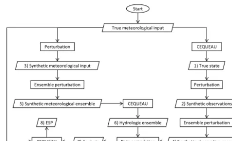
Figure 3.Flowchart for the production of ensemble streamflow pre-dictions obtained from various data assimilation scenarios.
between variables. The EnKF also assumes normally dis-tributed, bias-free and time-independent errors for both the model and the observations. Since these assumptions are not always met, which means that optimality is not guaranteed, a synthetic experiment is recommended to test the applicability of the method to the specific case being studied.
3 Experimental design 3.1 Synthetic experiment
Synthetic experiments, such as the ones done by Xie and Zhang (2010) or Weerts and El Serafy (2006), are test beds used to test the robustness of a data assimilation method or to tune various hyper-parameters. This is because the true state is known since it is initially created from true input that is also known.
to produce ESP (step 8) using the true meteorological input. Additional details pertaining to the procedure used in gener-ating perturbations and ensembles are included in the follow-ing sections.
3.1.1 Synthetic observation perturbation
Three types of observations were considered; namely stream-flow, SWE and SCA. These synthetic observations were gen-erated using a daily time step since their real-world counter-parts are usually available on a daily basis.
In order to abide by EnKF assumptions, observations er-rors should ideally have a normal distribution. However, this is not practical due to the physical limits of the observa-tions. For example, SWE observations cannot be negative and adding a normally distributed perturbation to SWE could result in some values being negative. Raising the negative values to zero or above would introduce a bias. Therefore, other distributions that share similarities with a normal dis-tribution, while ensuring that physical limits are respected, were used to generate synthetic observations.
Synthetic watershed-wide SCA were created using pertur-bations that follow a beta distribution since SCA is bounded between 0 and 1. SCA observations are expressed asyt,j∼ B−1 Qt,j|αt,j, βt,j
, whereQt,j is the cumulative
proba-bility of a temporally correlated normal random field with zero mean and unit variance at time t for observation j, and αt,j and βt,j are positively valued shape parameters.
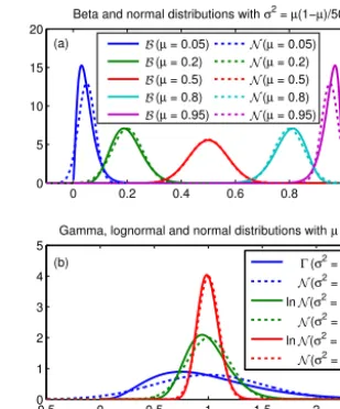
The shape parameters may be expressed in terms of the mean µt,j and varianceσt,j2 , but it must follow thatσt,j2 < µt,j 1−µt,j. The variance was arbitrarily set to σt,j2 = µt,j 1−µt,j/50, such that the resulting shape parameters
areαt,j=49µt,jandβt,j=49 1−µt,j. Examples of beta
distributions for different means using the same definition of variance as described above are shown in Fig. 4a. The distri-bution has a null variance and greater deviation from a nor-mal distribution when the snow covers either 0 or 100 % of the watershed, as well as a variance at its greatest and resem-bling most a normal distribution at 50 % SCA. This approach avoids introducing a systematic bias when assimilating ex-treme values of SCA. When values are at 0 % (or 100 %), perturbations can only introduce higher (or lower) values in order to remain within the physical limits of the observations. This approach also gives the observations a greater uncer-tainty during the transition periods when SCA is lower than 100 % and higher than 0 %, which loosely follows the greater uncertainty attributed to MODIS observations over the same periods (Hall and Riggs, 2007).
Synthetic streamflow and SWE observations were created using perturbations that have a lognormal distribution since both observations are bounded to the left at zero and are theo-retically unbounded to the right. Observation valuesyt,jcan
be expressed as yt,j ∼lnN−1
Qt,j|µt,j, σt,j2
. The true state was used forµt,j for both streamflow and SWE, while
0 0.2 0.4 0.6 0.8 1
0 5 10 15 20
Beta and normal distributions with σ2 = µ(1−µ)/50
(µ = 0.05)
(µ = 0.2)
(µ = 0.5)
(µ = 0.8)
(µ = 0.95)
(µ = 0.05)
(µ = 0.2)
(µ = 0.5)
(µ = 0.8)
(µ = 0.95)
−0.50 0 0.5 1 1.5 2 2.5
1 2 3 4 5
Gamma, lognormal and normal distributions with µ = 1
(σ2 = 0.5)
(σ2 = 0.5)
ln (σ2 = 0.2)
(σ2 = 0.2)
ln (σ2 = 0.1)
(σ2 = 0.1)
(a)
(b)
B B
B B B
N N N N N
Γ N
N
N N
[image:5.612.347.502.67.253.2]N
Figure 4.Examples of(a)beta and(b)gamma and lognormal dis-tribution compared with their analogous normal disdis-tributions using the same mean (µ) and variance (σ2).
the relative varianceσt,j2 was set to 20 and 10 % respectively. The error distributions using these parameters are shown in Fig. 4b. The exact value of these variances is arbitrary for feasibility purposes. However, since the conclusions of this study will likely be used to help set up real-world applica-tions, the variances chosen should ideally be relatively simi-lar to the error of their corresponding real observations. Since these real observation errors are not known, rough estimates are used.
The use of these distributions is a compromise between the normal distribution of observations required by the EnKF and the physical limits of the observations without introduc-ing a bias.
3.1.2 Meteorological input perturbation
Both the true daily precipitation and temperature values were perturbed using a gamma distribution, which has the benefit of generating positive values exclusively. Perturba-tions were implemented such that the meteorological input
zt,i (precipitation or temperature) at timet over the whole
squarei is the result of the inverse gamma function given the cumulative probability Pt,i of a spatially and
tempo-rally correlated normal random field with zero mean and unit variance. This can be expressed mathematically aszt,i∼ 0−1 Pt,i|κt,iθt,i, where κt,i andθt,i are shape and scale
factor respectively. The shape and scale factors can be ex-pressed in terms of meanµt,i and varianceσt,i2, such that κt,i=µ2t,i/ σt,i2 andθt,i=σt,i2 / µt,i. In this study, synthetic
precipitations are generated using the value of the true pre-cipitation forµt,i and a relative variance of 50 %, such that σt,i2 =0.5·µt,i. Figure 4 shows the resulting error
devia-tion of 1◦C. Within the synthetic study where the feasibility of the approach is tested, the exact value of these perturba-tions is arbitrary, so long as it is coherent between scenarios. The values used were such that the Nash–Sutcliffe efficiency (Nash and Sutcliffe, 1970) of the simulated streamflow re-sulting from CEQUEAU using the perturbed meteorologi-cal input compared with synthetic streamflow was roughly similar to the performance of the simulated streamflow using real-world meteorological input compared with real stream-flow observations.
3.1.3 Ensemble streamflow predictions generation
ESPs were generated using the ensemble of state variables resulting from the EnKF as initial states, true meteorologi-cal input and true model parameters. Using the true meteo-rological input implies that over a sufficiently large forecast horizon, every DA scenario considered in this study is likely to converge to the true state, but at different rates. By com-paring the relative gains in performance over the ensemble with no data assimilation (open loop), one can then observe the length of time upon which DA impacts ESPs without hav-ing erroneous meteorological input affecthav-ing the results. This still generates an ensemble of streamflows since each ensem-ble member has its own initial states (VOL, SWE, SRI, STI, SML, GWL, LWL).
ESPs were generated everyday over the entire study period (10 years) using a forecast horizon spanning 50 days.
3.2 Hyper-parameter tuning
The use of the EnKF requires the tuning of hyper-parameters, such as model and observation errors, and ensemble size. Im-proper specification of these hyper-parameters could lead to filter divergence (Houtekamer and Mitchell, 1998).
3.2.1 Ensemble size
The ensemble size should ideally approach infinity to reduce the impact of sampling when covariance matrices are com-puted, but this is not feasible given the limits of computing power and memory. In practice, the ensemble size is chosen such that computing time is more reasonable while ensuring that the sampling error remains small.
Tests were carried out using ensemble sizes of 8, 16, 32, 64 and 128 members. An ensemble size of 64 members was used for this study. This number was chosen as a function of the stability between successive runs and computing re-sources available. It was found to be a reasonable trade-off between having sufficiently consistent results between sim-ulations, such that the sampling error would be dwarfed in comparison with the impact of the actual data assimilation, without exceeding the computing resources available.
3.2.2 Meteorological ensemble generation
Perturbation factors similar to the ones used to generate syn-thetic meteorological inputs were used to generate an en-semble spread. This means that at every time step, meteo-rological ensemble (z0t,i) were generated using an inverse
gamma function given the cumulative probabilityP0t,i of a
spatially and temporally correlated normal random field with zero mean and unit variance, mathematically expressed as
z0t,i∼0−1 P0t,i|κ0t,i, θ0t,i
, where the shape factors are de-fined byκ0t,i=µ02t,i/ σ0
2
t,iandθ0t,i=σ02t,i/ µ0t,i. The prime
symbol is used to distinguish between the ensemble vari-ables/parameters and the synthetic varivari-ables/parameters. Pre-cipitation was generated using the value of the synthetic pre-cipitation (zt,i) forµ0t,iand a relative variance of 50 %, such
thatσ02t,i=0.5·zt,i, while temperature ensembles were
gen-erated using synthetic temperatures forµ0
t,i and a standard
deviation of 1◦C. Using similar perturbation factors between synthetic and ensemble versions of the meteorological input reduced the probability of filter divergence cause by a mis-representation of the model error. Errors from CEQUEAU-specific parameters were not taken into consideration, such that the parameter set used for the generation of the true state were the same for the ensemble generation.
3.2.3 Observation ensemble generation
As with model error representation, the perturbation fac-tors used to generate an ensemble of observations were similar to the ones used to generate synthetic observations. Streamflow and SWE observation ensembles were created using perturbations that have a lognormal distribution cen-tered around the synthetic observations zt,j with a
rela-tive variance of 20 and 10 % respecrela-tively. Watershed-wide SCA ensembles were created using a beta distribution cen-tered around the synthetic observationzt,j with a variance
ofσ02t,j=zt,j 1−zt,j
/50. Using similar perturbation fac-tors avoided problems caused by a misrepresentation of the observation errors.
3.2.4 Covariance localization
The main disadvantage in using a finite sample to compute covariance matrices is that the resulting covariance matrices are not exact. This may result in theoretically zero covariance elements between two theoretically uncorrelated variables to become small, but non-zero, which may deteriorate the per-formance of the EnKF.
in the covariance localization. This would further increase the number of parameters to set and the degree of subjectivity in setting those parameters when the degrees of dependence are unknown.
Another approach was used in this study, which is based on the improvements observed in the state vector. First, the open loop is executed, as well as a data assimilation scenario with one observation and the corresponding spatialized state variable included in the state vector (e.g. 1 snow pillow as-similated and all modelled SWE included in the state vector). Then, the two runs are compared with the true state on a spa-tial basis. In the case of CEQUEAU, these can be whole or partial squares depending on the variable analyzed. The co-variance matrix is localized such that the areas that do not show an improvement for the data assimilation scenario over the open loop are set to zero. This process is repeated for each observation.
While this process remains susceptible to the sampling er-ror from the finite ensemble size, it is a simple approach that exploits the availability of the true state in a synthetic exper-iment and limits the state vector size according to observed improvements.
In this study, only SWE observations have a correspond-ing state variable, so covariance localization has only been applied to the SWE variable.
3.2.5 State vector configuration
Though the state vector often comprises only of the variables corresponding to the observations or those judged to be rel-evant enough by the user, there are potentially many state variables that could benefit from the assimilation of available data if there exists a linear (or approximately linear) relation-ship between the modelled variables and the observations.
To determine which variable could benefit from being in-cluded in the state vector, one could execute multiple scenar-ios where each possible combination is compared with the true state. However, this could get very laborious even for a relatively small number of state variables. The current ap-proach suggests reducing this number by first adding state variables one at a time. The variables that show a global im-provement can then be added to the state vector. Assuming that not all variables are added to the state vector, this re-duces the number of combinations to try.
3.3 Metrics
Various metrics were used to quantify results. The mean square skill score (MSSS), based on the mean square error (MSE), was used to assess the differences between various data assimilation scenarios and the open loop during the state vector configuration and covariance localization processes. The MSE for a variable of interestxis defined as
MSE(x)= 1 N
N X
t=1
xt−xTt 2
, (6)
whereNis the number of time steps,xtis the ensemble mean
analysis of the state variable of interest at timet andxTt is the corresponding true state. It is often more convenient to express this score as a unitless skill score:
MSSS(x)=1− MSE(x)
MSEref(x)
, (7)
where MSEref(x) is a mean square error of reference; the
open loop in this case. The MSSS is bounded by [−∞,1] and indicates an improvement as the skill score increases. Values above zero indicate an improvement over the refer-ence (open loop) and a value of one indicates a perfect score: a perfect correspondence between the mean of the analysis and the true state.
The ensemble forecast performance was assessed using the continuous rank probability score (CRPS; Hersbach, 2000) and its associated skill score (CRPSS). For this syn-thetic study, the CRPS is adapted as follows:
CRPS(x, f )= 1 N
N X
t=1 +∞ Z
−∞
Fxft−F xTt2dx, (8)
whereFxft and F xTt are the cumulative distribution function of the ensemble forecast at a horizonf and the true state, respectively. The CRPS has the same units as the vari-able of interest and is bounded by [0,+∞]. A lower CRPS is a better score. As with the MSE and MSSS, it is often con-venient to express the CRPS in its skill score form:
CRPSS(x, f )=1− CRPS(x, f )
CRPSref(x, f )
, (9)
where CRPSref(xf )is the continuous rank probability score
of the open loop used as a reference in this case. Like the MSSS, the CRPSS is bounded by[−∞,1], with higher val-ues indicating a better score. Valval-ues above zero indicate an improvement over the reference and a value of one indicates a perfect score.
4 Results and discussion
4.1 State vector configuration and covariance localization
Before investigating the effect of data assimilation on stream-flow forecasts, a state vector configuration analysis was con-ducted. This was done in order to find out which variables, among the seven listed previously (VOL, SWE, SRI, STI, SML, GWL, LWL), should be included in the state vector for each type of data assimilated in order to reduce the num-ber of comparisons to make.
4.1.1 Streamflow data assimilation
VOL SWE SRI STI SML GWL LWL −1
−0.5 0 0.5 1
MSSS
[image:8.612.90.245.67.185.2]Streamflow data assimilation
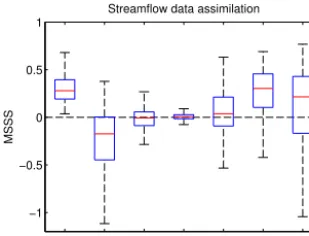
Figure 5.Box plot of the mean square skill score for each variable when assimilating streamflow at the outlet. The open loop is used as a reference. Outliers are not shown for visibility purposes.
outlet is computed by the model, but it is output only. There-fore, in order for the assimilation of streamflow to have any impact on the modelled states, additional variables needed to be added to the state vector.
Figure 5 shows a box plot of the MSSS computed for each variable on the whole watershed when they are individually included in the state vector using the open-loop scenario as a reference. Values above zero mean there is an improvement for a particular partial (for volumes) or whole (for other state variables) square compared with the open loop. The boxes range between the 25th and 75th percentiles, with a red bar to show the median, and the whiskers range between the max-imum and minmax-imum values. Outliers are not shown for vis-ibility purposes. Results for the case where water VOLs are included along with the streamflow at the outlet show an im-proved score for each partial square on the watershed. This is not entirely surprising given the close relationship between streamflow and volume. This suggests a necessity to include VOL in the state vector when assimilating streamflow at the outlet for streamflow predictions.
Results also show a deterioration of SWE for nearly 75 % of whole squares on the watershed. Although there is some improvement for some whole squares, this suggests that in-cluding SWE in the state vector when assimilating stream-flow at the outlet is unlikely to be beneficial for streamstream-flow predictions. Although SWE does have an important impact on streamflow, there is a time lag between the snowmelt oc-currence and the increase of streamflow at the outlet. Since the EnKF assumes linear relationships between variables, the non-linearity between SWE and streamflow can result in a non-optimal analysis. In this case, the results are ac-tually worse than open loop for most whole squares. Clark et al. (2008) discussed the issue of non-linearities between streamflow and other variables. To overcome this issue, one could use either a recursive approach, which allows for ad-justments of previously simulated variables, or a smoother approach to DA, which also uses “future” observations to up-date current state variables. However, this may not be neces-sary given the positive impact of streamflow DA on VOL, as
well as in a multivariate DA scenario where other variables, such as SWE in this case, are also assimilated.
As for the SRI and STI, the median sits around 0, which means there is no improvement for 50 % of the whole squares. This suggests little change can be obtained in the analysis by including those variables in the state vector. Sim-ilar to the case with SWE, there is likely a time lag issue be-tween streamflow and these variables. However, there is also a weaker link between these variables such that a change in SRI or STI is not as strongly linked to an eventual change in streamflow as much as it is for a change in SWE.
Finally, results for the three conceptual reservoirs SML, GWL and LWL show an improvement for over half of the whole squares, with a greater number of whole squares im-proved for the GWL and slightly above zero median for SML. This suggests that including these three variables in the state vector can potentially yield improvements for stream-flow predictions. Though the relationship between the wa-ter level in these conceptual reservoirs and streamflow at the outlet is not exactly linear, mainly due to reservoirs having multiple orifices (see Fig. 2) and the time lag before wa-ter reaches the outlet, it may be sufficiently near linear such that streamflow DA yields an overall improvement for most whole squares. For example, the median correlation coeffi-cient of a simple linear regression between each reservoir for each whole square and the streamflow at the outlet is 0.12, 0.49 and 0.15 for SML, GWL and LWL respectively.
Samuel et al. (2014) and Trudel et al. (2014) found that updating soil moisture with streamflow observations actu-ally deteriorated soil moisture simulation compared with real soil moisture observations. However, there are notable differ-ences between these studies and the present one. Aside from the different features of the study area and model structure, the use of synthetic data instead of real data likely strength-ens the link between variables and observations. Since syn-thetic observations are constructed using the same model and parameters as the model in which the observations are assim-ilated, there is no difference in scale between observations and modelled variables, which is often an important source of error for studies using real data.
Nonetheless, the inclusion of VOL, SML, GWL and LWL in the state vector were considered during the assimilation of streamflow at the outlet. The impact of each scenario for streamflow predictions are compared in Sect. 4.2.1.
4.1.2 SWE data assimilation
ex-Mount Wells
Mount Pondosy
Tahtsa Lake
1
0.5
0
-0.5
-1
20 30 40 50
20
15 25 30 35
I
J
1
0.5
0
-0.5
-1
20 30 40 50
20
15 25 30 35
I
J
1
0.5
0
-0.5
-1
20 30 40 50
20
15 25 30 35
I
J
(a)
(b)
[image:9.612.90.244.64.298.2](c)
Figure 6.Distribution of the mean square skill score of SWE over the watershed when assimilating SWE located at(a)Mount Wells, (b)Mount Pondosy and(c)Tahtsa Lake. The open loop is used as a reference. Values below−1 are cut off from the legend.
VOL SWE SRI STI SML GWL LWL −1
−0.5 0 0.5 1
MSSS
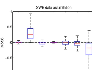
[image:9.612.350.506.68.185.2]SWE data assimilation
Figure 7.Box plot of the mean square skill score for each variable when assimilating SWE from all three snow pillow locations. The open loop is used as a reference. Outliers are not shown for visibility purposes.
tent upon which each snow pillow may affect modelled SWE in other whole squares.
Figure 6 shows the MSSS of SWE on the spatial level for the snow pillows located at Mount Wells, Mount Pondosy and Tahtsa Lake, using the open-loop scenario as a reference. For each figure, the whole square that shows the most im-provement is the area where the corresponding snow pillow is located. Whole squares that show improvements are mainly located around snow pillows, but the range differs for each snow pillows. Various areas in remote locations also show improvements for each snow pillow. As mentioned earlier, relationship with geophysical factors, such as distance from snow pillow, elevation and land cover, could be used to
ex-VOL SWE SRI STI SML GWL LWL
−10 −8 −6 −4 −2 0
MSSS
[image:9.612.91.247.373.491.2]SCA data assimilation
Figure 8.Box plot of the mean square skill score for each variable when assimilating basin-wide snow cover area. The open loop is used as a reference. Outliers are not shown for visibility purposes.
plain this variation, but a simpler approach was used such that the covariance localization was limited to whole squares showing improvements only. The covariance elements repre-senting all the other whole squares were set to zero.
As for the state vector configuration, Fig. 7 shows the MSSS computed for each variable within the extent of whole squares, which were positively impacted by SWE DA during the covariance localization process. The open-loop scenario was used again as a reference. The results show no signif-icant improvement for any other variable except for SWE itself, which yields only positive MSSS values by design. The lack of overall improvement for water-related variables (VOL, SML, GWL, LWL) is coherent with the time delay with changes in SWE. As for the other snow-related vari-ables (STI, SRI), although there may be a relationship with SWE, it is non-linear (US Army Corps of Engineers, 1956), which is further weakened by the distance separating SWE at a snow pillow from STI or SRI at another location.
Only the inclusion of SWE surrounding a given snow pil-low in the state vector is considered during the assimilation of SWE for streamflow predictions in Sect. 4.2.2.
4.1.3 SCA data assimilation
Like streamflow, SCA is not a state variable. It is computed in parallel with CEQUEAU without having any direct effect on future simulations. In order to have any impact during the assimilation process, there must exist a linear or sufficiently near-linear correlation between SCA and state variables. The update step should bring improvements to the state variables if the computed correlation also reflects the true correlation.
pur-0 10 20 30 40 50 −0.05
0 0.05 0.1 0.15 0.2 0.25 0.3 0.35 0.4
Forecast horizon (days)
CRPSS
Streamflow data assimilation
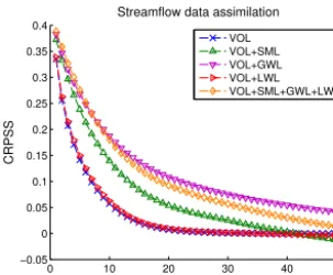
[image:10.612.91.243.66.191.2]VOL VOL+SML VOL+GWL VOL+LWL VOL+SML+GWL+LWL
Figure 9.Continuous rank probability skill score of the streamflow ensemble when assimilating streamflow at the outlet. The open loop is used as a reference. The forecast horizon varies from 1 to 50 days.
poses using the EnKF. Marcil et al. (2016) have shown that there exists a relationship between the SCA and the percent-age of cumulated streamflow at the outlet, but it is neither lin-ear nor is cumulated streamflow a state variable. The EnKF requirement that relationships between variables be linear and synchronized severely limits the value of global SCA data for the current application. This result is coherent with the findings presented by Clark et al. (2006). Using a model which incorporates snow cover area as a state variable, such as the snowmelt runoff model (SRM; Martinec, 1974) or the Soil and Water Assessment Tool (SWAT; Arnold et al., 1998), could overcome the issue of non-linearities between vari-ables, while using recursive or smoother approaches to data assimilation could help with the time lag issue between ob-servations and state variables.
Given the absence of overall improvement for all the state variables, the impact of SCA DA on streamflow predictions was not considered in this study.
4.2 Streamflow forecasts
Aside from granting insight into the sensitivity of the system to the state vector configuration, the analysis in the previous section presented a list of state vector configurations likely to favour streamflow predictions improvements based on the improvement of various state variables. This section presents ensemble streamflow prediction results for each configura-tion selected for each type of data assimilated.
4.2.1 Streamflow data assimilation
Focusing on the case where only streamflow at the outlet are assimilated, Fig. 9 presents the CRPSS of predicted stream-flow at the outlet over a forecast horizon of 50 days using the open loop as a reference. Only the state vector configu-rations that showed some improvements in the state vector configuration analysis section are shown.
First, high values of CRPSS for short-term forecasts can be observed for the case where only volumes are included in
the state vector (blue curve). The CRPSS subsides asymptoti-cally to zero over time, which shows assimilating streamflow to update volumes improves streamflow predictions com-pared to the open loop only for a few days, after which the impact of streamflow assimilation becomes insignificant. The duration of the impact depends on the residence time of the water stored in the model’s partial squares (VOL). A rel-atively short-lived impact would mean a relrel-atively short resi-dence time. The high initial impact is not surprising given the nearly linear relationship between streamflows and volumes. Assimilation of streamflow observations generate a globally positive update on volumes, as seen in Fig. 5, which in turn strongly affects simulated streamflows.
Second, adding each of the three water reservoirs individ-ually to the volumes yields different results. Even though lake water levels showed improvements over the majority of whole squares, the impact on streamflow predictions (red curve) is marginal compared to the case where only vol-umes are included in the state vector. This is because the weights attributed to lakes in CEQUEAU are very low for most whole squares. Only about 0.5 % of the entire water-shed is modelled using the conceptual lake reservoir and its parameters, unlike the soil moisture and groundwater reser-voirs, which are present in every whole square. Adding SML (green curve) or GWL (magenta curve) instead of LWL not only increases the initial CRPSS, but also slows the decrease over time. This is consistent with the improvements observed for the updated water levels for over half of the whole squares compared with the open-loop case, which translate as added improvements over the case where only volumes are included in the state vector. The slower decrease over time is also coherent with the increase in time it takes for water in the reservoirs to reach the outlet compared with water already in the routing system. The groundwater reservoir is shown to have an initially similar, but longer-lasting positive impact than the soil moisture reservoir. The soil moisture reservoir controls mainly the fast-flowing surface runoff, the amount of evapotranspiration leaving the system and the amount of water infiltrating into the groundwater reservoir. The ground-water reservoir has a numerically unlimited capacity, with no way out for the water except through evapotranspiration and the outlets that feed the routing system, making its impact on streamflows last longer than the relatively ephemeral soil moisture reservoir.
configuration analysis (Fig. 5), the assimilation of stream-flow at the outlet had a positive impact on a greater number of whole squares for the GWL than the SML. Here, the in-creased number of deteriorated SML, which infiltrates into the groundwater reservoirs, hinders the GWL updates such that the results show some deterioration compared with the VOL+GWL case, even though it is still an improvement over the VOL only updates.
These results have some similarities and differences with other studies. For example, Abaza et al. (2015) assimilated streamflow at the outlet using the EnKF to update two state variables (soil moisture in the intermediate and deep lay-ers of the hydrological model used in their study) using a time step of 3 h. The resulting gain in CRPS was high for the first time step and decreased quickly as a function of the forecast horizon such that mainly the first 24 h benefited from the data assimilation. Chen et al. (2013) found simi-lar results with multiple performance criteria when assimi-lating streamflow using a variant of the EnKF (the ensem-ble square root filter) to update various state variaensem-bles repre-sented by conceptual reservoirs. The observed improvement duration was even shorter, lasting less than 12 h during flash flood events. The difference in impact duration is likely re-lated to the different water retention time in each watershed. These studies were conducted on much smaller watersheds (all less than 800 km2) than the Nechako watershed (around 14 000 km2), further highlighting that the performance of as-similation techniques is related to watershed characteristics. 4.2.2 SWE data assimilation
Following the same method as with streamflow, this section focuses on the case where only SWE from snow pillows were assimilated. Since the state vector configuration anal-ysis showed only improvements for the SWE variable, it was the only variable added to the state vector for streamflow forecast. However, since there are three observations avail-able, Fig. 10 presents the CRPSS of predicted streamflow at the outlet when assimilating SWE from each snow pillow in-dividually and collectively.
An interesting result is that the impact of each snow pil-low on streamfpil-low predictions varies greatly. The impact of the snow pillows located at Mount Wells (green curve) and Mount Pondosy (blue curve) are dwarfed in comparison with the impact of the snow pillow located at Tahtsa Lake (ma-genta curve). This is coherent with results from Marcil et al. (2016) over the same watershed. The lower impact of the Mount Pondosy snow pillow is explained by the rela-tively small region of influence observed in Fig. 6b. As for Mount Well, even though it has the largest area of influence (Fig. 6a), it is also the snow pillow affecting the regions with the lowest altitudes and also the least amount of maximum SWE. Although the region affected by the Mount Wells snow pillow contains a mean annual maximum SWE of 410 mm, it is 40 % less than for the region affected by the Tahtsa Lake
0 10 20 30 40 50 0
0.05 0.1 0.15 0.2 0.25 0.3 0.35 0.4 0.45 0.5
Forecast horizon (days)
CRPSS
Snow water equivalent assimilation
[image:11.612.351.505.64.195.2]SWE (Mount Wells) SWE (Mount Pondosy) SWE (Tahtsa Lake) SWE (all)
Figure 10.Continuous rank probability skill score of the stream-flow ensemble when assimilating SWE from all three snow pillow locations. The open loop is used as a reference. The forecast horizon varies from 1 to 50 days.
0 10 20 30 40 50
0.4 0.42 0.44 0.46 0.48 0.5 0.52 0.54 0.56
Forecast horizon (days)
CRPSS
Streamflow and SWE data assimilation
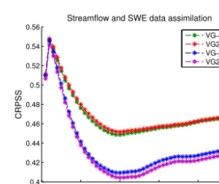
VG−S VG2−S VG−S2 VG2−S2
Figure 11.Continuous rank probability skill score of the streamflow ensemble when assimilating streamflow at the outlet and SWE from all three snow pillow locations. The open loop is used as a reference. The forecast horizon varies from 1 to 50 days. Lack of parentheses indicates that the variable is affected by both types of observations.
snow pillow, which contains a mean annual maximum SWE of 682 mm.
[image:11.612.350.504.270.399.2]Table 1.Overview of multivariate DA scenarios.
Streamflow DA updates SWE DA updates:
Method VOL+GWL? SWE? VOL+GWL? SWE?
VG-S yes no no yes
VG2-S yes no yes yes
VG-S2 yes yes no yes
VG2-S2 yes yes yes yes
Franz et al. (2014) also assessed the impact of SWE data assimilation on ensemble predictions, but using real obser-vations. Their results showed little improvement of forecast performance through SWE data assimilation, but they high-lighted the role of a possible bias in the observations, as well as the difference in scale between the point-scale observa-tions and the basin average SWE simulated by the model. In this synthetic experiment, no bias was specified on observa-tions and there is no difference in scale between modelled and observed SWE, which could explain the differences ob-served between the two studies. Biased observations and me-teorological input were purposely omitted in this study, but may be added in future works to test the robustness of the approach.
4.2.3 Combined streamflow and SWE data assimilation The focus now shifts to the case where streamflow at the outlet are simultaneously assimilated along with SWE from the three snow pillows. The state vector configuration, which provided the best results from the streamflow data assimila-tion case, is used (VOL+GWL) along with the best config-uration from SWE data assimilation (SWE only). Although these configurations worked best with their respective data assimilation case, they could behave differently when both streamflow and SWE are assimilated together.
Table 1 presents four configurations for the combined as-similation of streamflow and SWE observations. These con-figurations differ in the overlap of their effect during the up-date phase such that some configurations allow both observa-tions to simultaneously update the same variable, while oth-ers do not.
The performance of these configurations on the CRPSS for predicted streamflow at the outlet is presented in Fig. 11. While all four configurations perform in a very similar way for short-term streamflow predictions, the group forms two pairs that differ in that the blue-magenta group allows SWE observations to update modelled streamflow, while the green-red pair does not. Although allowing SWE data assimilation to update VOL and GWL changes very little, a drop in per-formance occurs if streamflow assimilation updates modelled SWE. This is coherent with the state vector configuration analysis performed in the previous section (Figs. 5 and 7), where SWE data assimilation is shown to have a weak im-pact on VOL and a median MSSS around 0 for GWL, while
Jan Mar May Jul Sep Nov
0 5 10 15 20 25 30 35 40 45 50
Month of the year
CRPS
Short-term forecasts (days 1−5 average)
Open loop Streamflow DA SWE DA Streamflow+SWE DA
Figure 12.Continuous rank probability score for short-term fore-casts (average of forecast horizons 1 through 5 days) of various data assimilation scenarios as a function of the month of the year.
Jan Mar May Jul Sep Nov
0 5 10 15 20 25 30 35 40 45
Month of the year
CRPS
Mid-term forecasts (days 25−50 average)
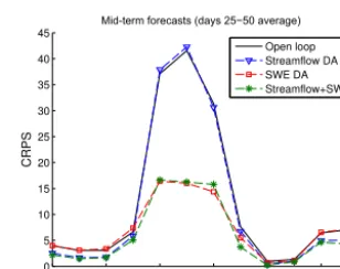
[image:12.612.55.276.84.152.2]Open loop Streamflow DA SWE DA Streamflow+SWE DA
Figure 13.Continuous rank probability score for mid-term fore-casts (average of forecast horizons 25 through 50 days) of various data assimilation scenarios as a function of the month of the year.
streamflow assimilation deteriorated around 75 % of SWE whole squares when they were included in the state vector.
Overall, the simultaneous assimilation of streamflow and observed SWE yields important improvements over the en-tire forecast horizon analyzed, with the streamflow data assimilation improving mainly short-term streamflow fore-casts and SWE data assimilation improving mainly mid-term streamflow forecasts. CRPSS values for combined assimila-tion of both streamflow and SWE observaassimila-tions were supe-rior to CRPSS values for individual assimilation of stream-flow or SWE over all forecast horizons, with the exception of forecast horizons higher than 45 days, where CRPSS values for SWE DA are slightly higher. This reveals that the up-dated VOL and GWL by streamflow data assimilation may be very beneficial for short-term forecasts; furthermore, they do not further improve the mid-term forecasts when com-bined with SWE data assimilation in comparison with the scenario where only SWE data are assimilated.
[image:12.612.351.505.255.377.2]curve), the SWE data assimilation of all snow pillows (red curve) and the simultaneous, but separated, streamflow and SWE data assimilation (VG-S; green curve) for short-term (average of horizon from 1 to 5 days) and mid-term (aver-age of horizon from 25 to 50 days) streamflow forecasts. The CRPS is shown for the open loop to show the performance change over the time of the year and the period when im-provement is most needed. Recall that the CRPS ranges from zero to infinity, with zero being a perfect forecast. The period from May to July, which corresponds to the melt period, is therefore the period when the CRPS is the highest for short-and mid-term forecasts are the most problematic. The scores for mid-term forecasts are lower than for short-term forecasts because the true weather is used as input for forecasts such that the open loop slowly converges to the true states over time.
Assimilating streamflow results in an improved score over the entire year for short-term forecasts, although little gain is obtained for mid-term forecasts. This steady improvement is to be expected since streamflow here is always non-zero and observations are available all-year round. On the other hand, the impact of the assimilation SWE from snow pillows is limited mainly to the melt period for both short-term and mid-term forecasts. However, this period corresponds to the problematic period when most gain can be obtained. The as-similation of SWE provides a better score than the assimi-lation of streamflow for the same period and improves go-ing from short-term to mid-term forecasts. SWE assimilation complements streamflow assimilation as observed from the performance of the simultaneous assimilation, which yields both the steady improvements over the year and the impor-tant gain during the snowmelt period.
5 Conclusion
This study investigated the impact that multivariate data as-similation can have on streamflow forecasts using the CE-QUEAU hydrologic model applied over the Nechako water-shed in a synthetic experiment. The study also showed the importance of the state vector configuration on streamflow forecasts when using the EnKF.
Streamflow data assimilation was found to improve short-term streamflow forecast considerably. However, the impact dissipated relatively rapidly as a function of the forecast hori-zon, which was slowed by adding groundwater conceptual reservoir levels to the state vector. Improvements were ob-served for all months of the year: low-flow and high-flow periods alike.
On the other hand, the assimilation of snow water equiva-lent data from synthetic snow pillow data yielded streamflow forecast improvements mainly during the snowmelt period. Although the period lasts approximately 3 months, the im-pact was found to be greater than streamflow data assimila-tion over the same period. It was also noted that
assimilat-ing each snow pillow data individually yielded different re-sults, with various radii of influence, such that the improve-ment from assimilating all three snow pillows simultaneously covered most of the watershed and yielded streamflow fore-casts which outperformed forefore-casts from any single snow pil-low data assimilation. Over the forecast horizon, the peak of improvement was greater than or equal to the 50-day limit over which forecasts were simulated, which contrasts with the short-lived impact of streamflow data assimilation.
Given their complementarity, streamflow and snow wa-ter equivalent data were assimilated simultaneously. The re-sulting streamflow forecast inherited the strengths from both types of data, having a strong, positive impact for both short-term and mid-short-term forecasts. Improvements were obtained for all periods of the year, but mainly during the snowmelt period, which is normally the most problematic.
The assimilation of basin-wide snow cover area failed to improve the simulation of any state variable. The most prob-able factor was determined to be the absence of snow cover area as a state variable or a proxy with a sufficiently linear relationship with SCA. Suggestions to improve the method to accommodate for snow cover area are to use a model that incorporates snow cover area as a state variable and/or to use a data assimilation approach, which takes into account a time lag between observations and state variables.
The results obtained are conditional to some assump-tions and limitaassump-tions. First, all results depend on the gen-eral method and parameters used in creating the synthetic framework. Since this is a synthetic experiment, it is as-sumed that a real experiment would behave similarly to a simulation using CEQUEAU with a specific set of parame-ters and inputs. Second, the potential impact of data assimila-tion on streamflow forecasts observed depended on using the true weather inputs. Using real weather inputs may decrease this impact. Third, it is assumed that the error representations for the model inputs and the observations are known. In this study, they have been generated using specific distributions and variances to compromise between the need for normal distributions and the need to remain within the physical lim-its of the variables without introducing a bias. Finally, the impact of errors from the model parameters is assumed to be negligible, such that the set of parameters was not altered from the true simulation’s set of parameters.
6 Data availability
The synthetic meteorological input and observations used in this study are available at https://dx.doi.org/10.6084/m9. figshare.4057653.v1.
Acknowledgements. We thank Rio Tinto for their collaboration in this study, providing funding, data and the hydrologic model CE-QUEAU. This research is also supported by the funding agencies FRQNT, Quebec, and NSERC, Canada. We are also grateful for the two anonymous referees and Kevin He for taking the time to provide constructive comments.
Edited by: F. Pappenberger
Reviewed by: K. He and two anonymous referees
References
Abaza, M., Anctil, F., Fortin, V., and Turcotte, R.: Se-quential streamflow assimilation for short-term hydrolog-ical ensemble forecasting, J. Hydrol., 519, 2692–2706, doi:10.1016/j.jhydrol.2014.08.038, 2014.
Abaza, M., Anctil, F., Fortin, V., and Turcotte, R.: Ex-ploration of sequential streamflow assimilation in snow dominated watersheds, Adv. Water Resour., 80, 79–89, doi:10.1016/j.advwatres.2015.03.011, 2015.
Anderson, E. A.: National Weather Service river forecast system: Snow accumulation and ablation model, US Department of Com-merce, National Oceanic and Atmospheric Administration, Na-tional Weather Service, Washington, D.C., 240 pp., 1973. Andreadis, K. M. and Lettenmaier, D. P.: Assimilating
re-motely sensed snow observations into a macroscale hydrology model, Adv. Water Resour., 29, 872–886, doi:10.1016/j.advwatres.2005.08.004, 2006.
Arnold, J. G., Srinivasan, R., Muttiah, R. S., and Williams, J. R.: Large Area Hydrologic Modeling and Assessment Part I: Model Development, J. Am. Water Resour. Assoc., 34, 73–89, doi:10.1111/j.1752-1688.1998.tb05961.x, 1998.
Bergeron, J., Royer, A., Turcotte, R., and Roy, A.: Snow cover estimation using blended MODIS and AMSR-E data for improved watershed-scale spring streamflow simula-tion in Quebec, Canada, Hydrol. Process., 28, 4626–4639, doi:10.1002/hyp.10123, 2014.
Charbonneau, R., Fortin, J.-P., and Morin, G.: The CEQUEAU Model: Description and Examples of its use in Problems Related to Water Resource Management, Hydrol. Sci. Bull., 22, 193–202, doi:10.1080/02626667709491704, 1977.
Chen, H., Yang, D., Hong, Y., Gourley, J. J., and Zhang, Y.: Hydro-logical data assimilation with the Ensemble Square-Root-Filter: Use of streamflow observations to update model states for real-time flash flood forecasting, Adv. Water Resour., 59, 209–220, doi:10.1016/j.advwatres.2013.06.010, 2013.
Clark, M. P., Slater, A. G., Barrett, A. P., Hay, L. E., Mc-Cabe, G. J., Rajagopalan, B., and Leavesley, G. H.: As-similation of snow covered area information into hydrologic and land-surface models, Adv. Water Resour., 29, 1209–1221, doi:10.1016/j.advwatres.2005.10.001, 2006.
Clark, M. P., Rupp, D. E., Woods, R. a., Zheng, X., Ibbitt, R. P., Slater, A. G., Schmidt, J., and Uddstrom, M. J.: Hy-drological data assimilation with the ensemble Kalman fil-ter: Use of streamflow observations to update states in a dis-tributed hydrological model, Adv. Water Resour., 31, 1309– 1324, doi:10.1016/j.advwatres.2008.06.005, 2008.
Day, G. N.: Extended Streamflow Forecasting Using NWS-RFS, J. Water Resour. Plan. Manag., 111, 157–170, doi:10.1061/(ASCE)0733-9496(1985)111:2(157), 1985. Dechant, C. M. and Moradkhani, H.: Improving the
characteriza-tion of initial condicharacteriza-tion for ensemble streamflow prediccharacteriza-tion us-ing data assimilation, Hydrol. Earth Syst. Sci., 15, 3399–3410, doi:10.5194/hess-15-3399-2011, 2011.
De Lannoy, G. J. M., Reichle, R. H., Arsenault, K. R., Houser, P. R., Kumar, S., Verhoest, N. E. C., and Pauwels, V. R. N.: Multiscale assimilation of Advanced Microwave Scanning Radiometer-EOS snow water equivalent and Moderate Reso-lution Imaging Spectroradiometer snow cover fraction obser-vations in northern Colorado, Water Resour. Res., 48, 1–17, doi:10.1029/2011WR010588, 2012.
De Roo, A. P. J., Gouweleeuw, B., Thielen, J., Bartholmes, J., Bongioannini-Cerlini, P., Todini, E., Bates, P. D., Horritt, M., Hunter, N., Beven, K., Pappenberger, F., Heise, E., Rivin, G., Hils, M., Hollingsworth, A., Holst, B., Kwadijk, J., Reggiani, P., Van Dijk, M., Sattler, K., and Sprokkereef, E.: Development of a European flood forecasting system, Int. J. River Basin Manag., 1, 49–59, doi:10.1080/15715124.2003.9635192, 2003.
Duan, Q. Y., Sorooshian, S., and Gupta, V.: Effective and Efficient Global Optimization for Conceptual Rainfall-Runoff Models, Water Resour. Res., 28, 1015–1031, doi:10.1029/91wr02985, 1992.
Evensen, G.: Sequential data assimilation with a nonlinear quasi-geostrophic model using Monte Carlo methods to forecast error statistics, J. Geophys. Res., 99, 10143, doi:10.1029/94JC00572, 1994.
Evensen, G.: The Ensemble Kalman Filter: Theoretical formula-tion and practical implementaformula-tion, Ocean Dynam., 53, 343–367, doi:10.1007/s10236-003-0036-9, 2003.
Evensen, G. and van Leeuwen, P. J.: An Ensemble Kalman Smoother for Nonlinear Dynamics, Mon. Weather Rev., 128, 1852–1867, doi:10.1175/1520-0493(2000)128<1852:AEKSFN>2.0.CO;2, 2000.
Franz, K. J., Hogue, T. S., and Sorooshian, S.: Snow Model Verifi-cation Using Ensemble Prediction and Operational Benchmarks, J. Hydrometeorol., 9, 1402–1415, doi:10.1175/2008JHM995.1, 2008.
Franz, K. J., Hogue, T. S., Barik, M., and He, M.: Assessment of SWE data assimilation for ensemble streamflow predictions, J. Hydrol., 519, 2737–2746, doi:10.1016/j.jhydrol.2014.07.008, 2014.
Hall, D. K. and Riggs, G. A.: Accuracy assessment of the MODIS snow products, Hydrol. Process., 21, 1534–1547, doi:10.1002/hyp.6715, 2007.
Hall, D. K., Riggs, G. A., Salomonson, V. V., DiGirolamo, N. E., and Bayr, K. J.: MODIS snow-cover products, Remote Sens. Environ., 83, 181–194, doi:10.1016/S0034-4257(02)00095-0, 2002.
ap-proach for improved operational streamflow predictions, Hydrol. Earth Syst. Sci., 16, 815–831, doi:10.5194/hess-16-815-2012, 2012.
Houtekamer, P. L. and Mitchell, H. L.: Data assimi-lation using an ensemble Kalman filter technique, Mon. Weather Rev., 126, 796–811, doi:10.1175/1520-0493(1998)126<0796:DAUAEK>2.0.CO;2, 1998.
Houtekamer, P. L. and Mitchell, H. L.: A Sequential En-semble Kalman Filter for Atmospheric Data Assimilation, Mon. Weather Rev., 129, 123–137, doi:10.1175/1520-0493(2001)129<0123:ASEKFF>2.0.CO;2, 2001.
Lee, H., Seo, D. J., and Koren, V.: Assimilation of streamflow and in situ soil moisture data into operational distributed hy-drologic models: Effects of uncertainties in the data and initial model soil moisture states, Adv. Water Resour., 34, 1597–1615, doi:10.1016/j.advwatres.2011.08.012, 2011.
Liu, Y. and Gupta, H. V.: Uncertainty in hydrologic modeling: To-ward an integrated data assimilation framework, Water Resour. Res., 43, 1–18, doi:10.1029/2006WR005756, 2007.
Liu, Y., Weerts, A. H., Clark, M., Hendricks Franssen, H. J., Kumar, S., Moradkhani, H., Seo, D. J., Schwanenberg, D., Smith, P., Van Dijk, A. I. J. M., Van Velzen, N., He, M., Lee, H., Noh, S. J., Rakovec, O., and Restrepo, P.: Advancing data assimilation in operational hydrologic forecasting: Progresses, challenges, and emerging opportunities, Hydrol. Earth Syst. Sci., 16, 3863–3887, doi:10.5194/hess-16-3863-2012, 2012.
Marcil, G.-K., Leconte, R., and Trudel, M.: Using Remotely Sensed MODIS Snow Product for the Management of Reservoirs in a Mountainous Canadian Watershed, Water Resour. Manag., Ac-cepted, 2016.
Martinec, J.: Snowmelt – Runoff Model For Stream Flow Forecasts, Nord. Hydrol., 6, 145–154, 1974.
McMillan, H. K., Hreinsson, E. O., Clark, M. P., Singh, S. K., Za-mmit, C., and Uddstrom, M. J.: Operational hydrological data assimilation with the recursive ensemble Kalman filter, Hydrol. Earth Syst. Sci., 17, 21–38, doi:10.5194/hess-17-21-2013, 2013.
Nagler, T., Rott, H., Malcher, P., and Muller, F.: Assimila-tion of meteorological and remote sensing data for snowmelt runoff forecasting, Remote Sens. Environ., 112, 1408–1420, doi:10.1016/j.rse.2007.07.006, 2008.
Nash, J. E. and Sutcliffe, J. V.: River flow forecasting through con-ceptual models part I – A discussion of principles, J. Hydrol., 10, 282–290, doi:10.1016/0022-1694(70)90255-6, 1970.
Roy, A., Royer, A., and Turcotte, R.: Improvement of springtime streamflow simulations in a boreal environment by incorporating snow-covered area derived from remote sensing data, J. Hydrol., 390, 35–44, doi:10.1016/j.jhydrol.2010.06.027, 2010.
Samuel, J., Coulibaly, P., Dumedah, G., and Moradkhani, H.: Assessing model state and forecasts variation in hy-drologic data assimilation, J. Hydrol., 513, 127–141, doi:10.1016/j.jhydrol.2014.03.048, 2014.
Slater, A. G. and Clark, M. P.: Snow Data Assimilation via an Ensemble Kalman Filter, J. Hydrometeorol., 7, 478–493, doi:10.1175/JHM505.1, 2006.
Tang, Q. and Lettenmaier, D. P.: Use of satellite snow-cover data for streamflow prediction in the Feather River Basin, California, Int. J. Remote Sens., 31, 3745–3762, doi:10.1080/01431161.2010.483493, 2010.
Trudel, M., Leconte, R., and Paniconi, C.: Analysis of the hy-drological response of a distributed physically-based model us-ing post-assimilation (EnKF) diagnostics of streamflow and in situ soil moisture observations, J. Hydrol., 514, 192–201, doi:10.1016/j.jhydrol.2014.03.072, 2014.
US Army Corps of Engineers: Snow Hydrology, Summary report of the snow investigation, North Pacific Division, Portland, Oregon, 437 pp., 1956.
Weerts, A. H. and El Serafy, G. Y. H.: Particle filtering and ensem-ble Kalman filtering for state updating with hydrological con-ceptual rainfall-runoff models, Water Resour. Res., 42, 1–17, doi:10.1029/2005WR004093, 2006.