Response of water temperatures and stratification to changing climate in three lakes with different morphometry

https://doi.org/10.5194/hess-21-6253-2017 © Author(s) 2017. This work is distributed under the Creative Commons Attribution 3.0 License.

Response of water temperatures and stratification to changing

climate in three lakes with different morphometry

Madeline R. Magee1,2and Chin H. Wu1

1_{Department of Civil and Environmental Engineering, University of Wisconsin-Madison,}

Madison, WI 53706, USA

2_{Center of Limnology, University of Wisconsin-Madison, Madison, WI 53706, USA}

Correspondence:Chin H. Wu ([email protected]) Received: 27 May 2016 – Discussion started: 26 July 2016

Revised: 13 October 2017 – Accepted: 2 November 2017 – Published: 11 December 2017

Abstract. Water temperatures and stratification are impor-tant drivers for ecological and water quality processes within lake systems, and changes in these with increases in air temperature and changes to wind speeds may have signifi-cant ecological consequences. To properly manage these sys-tems under changing climate, it is important to understand the effects of increasing air temperatures and wind speed changes in lakes of different depths and surface areas. In this study, we simulate three lakes that vary in depth and sur-face area to elucidate the effects of the observed increasing air temperatures and decreasing wind speeds on lake thermal variables (water temperature, stratification dates, strength of stratification, and surface heat fluxes) over a century (1911– 2014). For all three lakes, simulations showed that epilim-netic temperatures increased, hypolimepilim-netic temperatures de-creased, the length of the stratified season increased due to earlier stratification onset and later fall overturn, stability in-creased, and longwave and sensible heat fluxes at the sur-face increased. Overall, lake depth influences the presence of stratification, Schmidt stability, and differences in surface heat flux, while lake surface area influences differences in hypolimnion temperature, hypolimnetic heating, variability of Schmidt stability, and stratification onset and fall overturn dates. Larger surface area lakes have greater wind mixing due to increased surface momentum. Climate perturbations indi-cate that our larger study lakes have more variability in tem-perature and stratification variables than the smaller lakes, and this variability increases with larger wind speeds. For all study lakes, Pearson correlations and climate perturbation scenarios indicate that wind speed has a large effect on tem-perature and stratification variables, sometimes greater than

changes in air temperature, and wind can act to either amplify or mitigate the effect of warmer air temperatures on lake ther-mal structure depending on the direction of local wind speed changes.

1 Introduction

The past century has experienced global changes in air tem-perature and wind speed. Land and ocean surface tempera-ture anomalies relative to 1961–1990 increased from 1850 to 2012 (IPCC, 2013). Mean temperature anomaly across the continental United States has increased (Hansen et al., 2010), and studies suggest that more intense and longer lasting heat waves will continue in the future (Meehl and Tebaldi, 2004). Additionally, global change in wind speed has been het-erogenous. For example, wintertime wind energy increased in northern Europe (Pryor et al., 2005), but other parts of Europe have experienced decreases in wind speed in part due to increased surface roughness (Vautard et al., 2010), while modest declines in mean wind speeds were observed in the United States (Breslow and Sailor, 2002). Similarly, on regional scales, Magee et al. (2016) showed a decrease in Madison, Wisconsin, wind speeds after 1994, but Austin and Colman (2007) found increased wind speeds in Lake Supe-rior, North America. Significant changes to air temperature and wind speed observed in the contemporary and historical periods are likely to continue to change in the future.

water temperatures (Dobiesz and Lester, 2009; Ficker et al., 2017; O’Reilly et al., 2015; Shimoda et al., 2011), increased strength of stratification (Hadley et al., 2014; Rempfer et al., 2010), prolonged stratified period (Ficker et al., 2017; Liv-ingstone, 2003; Woolway et al., 2017a), and altered ther-mocline depth (Schindler et al., 1990). However, hypolim-netic temperatures have undergone warming, cooling, and no temperature increase (Butcher et al., 2015; Ficker et al., 2017; Magee et al., 2016; Shimoda et al., 2011). Wind speed also strongly affects lake mixing (Boehrer and Schultze, 2008), lake heat transfer (Boehrer and Schultze, 2008; Read et al., 2012), and temperature structure (Desai et al., 2009; Schindler et al., 1990). Stefan et al. (1996) found that de-creasing wind speeds resulted in increased stratification and increased epilimnetic temperatures in inland lakes. Similarly, Woolway et al. (2017a) found that decreasing wind speeds increased days of stratification for a polymictic lake in Eu-rope. In Lake Superior, observations show that the com-plex non-linear interactions among air temperature, ice cover, and water temperature result in water temperature increases (Austin and Allen, 2011), contrary to the expected decreases in water temperature from increased wind speeds (Desai et al., 2009). In recent years, our understanding of the effects of air temperature and wind speed on changes in water temper-ature and stratification has improved (Kerimoglu and Rinke, 2013; Magee et al., 2016; Woolway et al., 2017a), but re-search on the response of lakes to isolated and combined changes in air temperature and wind speed has been limited. Changes in lake water temperature influence lake ecosys-tem dynamics (MacKay et al., 2009). For example, increas-ing water temperatures may change plankton community composition and abundance (Rice et al., 2015), alter fish pop-ulations (Lynch et al., 2015), and enhance the dominance of cyanobacteria (Jöhnk et al., 2008). Such changes affect the biodiversity of freshwater ecosystems (Mantyka-Pringle et al., 2014). Furthermore, increased thermal stratification of lakes can intensify lake anoxia (Ficker et al., 2017; Palmer et al., 2014), increase bloom-forming cyanobacteria (Paerl and Paul, 2012), and change internal nutrient loading and lake productivity (Ficker et al., 2017; Verburg and Hecky, 2009). Variations in water temperature impact the distribution, be-havior, community composition, reproduction, and evolu-tionary adaptations of organisms (Thomas et al., 2004). Im-proved understanding of the response of lake water temper-atures and ecosystem response to air temperature and wind speed can better prepare management, adaptation, and miti-gation efforts for a range of lakes.

Lake morphometry complicates the response of lake wa-ter temperatures to air temperature and wind speed changes because it alters physical processes of wind mixing, water circulation, and heat storage (Adrian et al., 2009). Mean depth, surface area, and volume strongly affect lake strati-fication (Butcher et al., 2015; Kraemer et al., 2015). Large surface areas increase the effects of vertical wind mixing, an important mechanism for transferring heat to the lake

bot-tom (Rueda and Schladow, 2009), and changes in thermo-cline depth from warming air temperatures may be damp-ened in large lakes where thermocline depth is constrained by lake fetch (Boehrer and Schultze, 2008; MacIntyre and Melack, 2010). Lake size has been demonstrated to influ-ence the relative contribution of wind and convective mixing to gas transfer (Read et al., 2012), and lake size can influ-ence the magnitude of diurnal heating and cooling in lakes (Woolway et al., 2016), which both have implications for cal-culating metabolism and carbon emissions in inland waters (Holgerson et al., 2017). Winslow et al. (2015) showed that differences in wind-driven mixing may explain the inconsis-tent response of hypolimnetic temperatures between small and large lakes. Previous research efforts have investigated the response of individual lakes (Voutilainen et al., 2014) and the bulk response of lakes in a geographic region to chang-ing climate (Kirillin, 2010; Magnuson et al., 1990), but few studies have focused on elucidating the effects of morphom-etry, specifically lake depth and surface area, on changes in lake water temperature in response to long-term changes in air temperature and wind speed.

The purpose of this paper is to investigate the response of water temperatures and stratification in lakes with differ-ent morphometry (water depth and surface area) to chang-ing air temperature and wind speed. To do this, we employ an existing one-dimensional hydrodynamic lake-ice model to hindcast water temperatures for three lakes with different morphometry. These lakes vary in surface area and depth and are near one another (< 30 km distance) to experience similar daily climate conditions (air temperature, wind speed, solar radiation, cloud cover, precipitation) over the century period (1911–2014). By examining three lakes in the same ecore-gion with similar climate forcing, we aim to elucidate dif-ferences in responses that relate to morphometry rather than climatic variables. Long-term changes in water temperature, stratification, heat fluxes, and stability are used to investigate how lake depth and surface area alter the response of thermal structure to air temperature and wind speed changes for the three study lakes.

2 Methods 2.1 Study sites

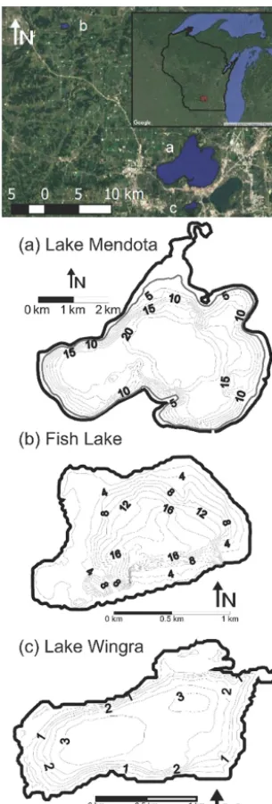
Three morphometrically different lakes, Lake Mendota, Fish Lake, and Lake Wingra, located near Madison, Wisconsin, United States of America (USA), were selected for this study. These lakes are chosen for (i) their morphometry differences, (ii) their proximity to one another, and (iii) the availability of long-term data for model input and calibration.

peri-Figure 1.(Top) map of study lakes in Wisconsin, USA and bathy-metric maps of each lake: (a) Lake Mendota, (b) Fish Lake, and(c)Lake Wingra.

ods last from May to September. Summer (1 June–31 Au-gust) mean surface water temperature is 22.4◦C, and hy-polimnetic temperatures vary between 11 and 15◦C. Nor-mal Secchi depth during the summer is 3.0 m (Lathrop et al., 1996). Fish Lake (43◦₁₇0_{N; 89}◦₃₉0_{W; Fig. 1b; Table 1) is}

a dimictic, eutrophic, shallow seepage lake located in north-western Dane County. From 1966 to 2001, the lake level rose by 2.75 m due to increased groundwater flow from higher-than-normal regional groundwater recharge (Krohelski et al., 2002). Krohelski et al. (2002) hypothesized that the increase in recharge may be the result of increased infiltration from snowmelt after increased snowfall and less frost-covered soil.

Summer stratification lasts from the beginning of May to mid-September. Mean surface water temperature is 23.9◦_C,

and hypolimnetic temperatures are normally near 8◦_{C during}

the summer months; however, some years reach temperatures of only 5–6◦C in the hypolimnion due to shortened spring mixing durations. Average Secchi depth during the summer months is 2.4 m. Lake Wingra (43◦30N; 89◦260W; Fig. 1c; Table 1) is a shallow eutrophic drainage lake. It stratifies on short timescales of hours to weeks (Kimura et al., 2016) but does not experience sustained thermal stratification. Summer mean water temperature is 23.9◦C, and mean Secchi depth is 0.7 m. All three lakes have ice cover during the winter months, and a description of ice on the lakes can be found in Magee and Wu (2017).

2.2 Model description

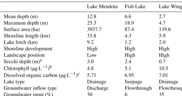
pe-Table 1.Lake characteristics for the three study lakes.

Lake Mendota Fish Lake Lake Wingra

Mean depth (m) 12.8 6.6 2.7

Maximum depth (m) 25.3 18.9 4.7

Surface area (ha) 3937.7 87.4 139.6

Shoreline length (km) 33.8 4.3 5.9

Lake fetch (km) 9.2 1.2 2.0

Shoreline development High High High

Landscape position Low High High

Secchi depth (m)a 3.0 2.4 0.7

Chlorophyll (µg L−1)b 4.8 5.1 10.5 Dissolved organic carbon (µg L−1)c 5.71 6.95 7.01

Lake type Drainage Seepage Drainage

Groundwater inflow type Discharge Flowthrough Flowthrough

Groundwater input (%) 30 6 35

a_{Secchi depth measured from 1 June to 31 August.}b_{Surface chlorophyll from the open-water season.}c_Dissolved

organic carbon is the average of all measurements for each lake.

riod. Yeates and Imberger (2003) improved performance of the surface mixed layer routine within the model by includ-ing an effective surface area algorithm based on observa-tions in five lakes of different size, shape, and wind forc-ing characteristics (see Eq. 32 in Yeates and Imberger, 2003) that reduced surface mixing in smaller, more sheltered lakes. The effective area is used to modify the transfer of mo-mentum from surface stress, as described in detail in Yeates and Imberger (2003) and not reproduced here. Their analy-sis developed a strong inverse relationship between the lake number and lake-wide average vertical eddy diffusion co-efficient, which configures a pseudo two-dimensional deep mixing within the code, found to significantly improve the simulation of thermal structures observed in lakes that ex-perienced strong wind forcing (Yeates and Imberger, 2003). Details of the surface mixed layer algorithm are not repro-duced here but can be found in Eqs. (27)–(34) of Yeates and Imberger (2003). Hypolimnetic mixing is parameterized through a vertical eddy diffusion coefficient, which accounts for turbulence created by the damping of basin-scale inter-nal waves on the bottom boundary and lake interior (Yeates and Imberger, 2003). Detailed equations on the simulation of water temperature and mixing can be found in Imberger and Patterson (1981), Imerito (2010), and Yeates and Im-berger (2003).

Sediment heat flux is included as a source/sink term for each model layer. A diffusion relation from Rogers et al. (1995) is used to estimateqsed, heat transfer from the

sed-iments to the water column. qsed=Ksed

dT

dz, (1)

whereKsedrepresents the sediment conductivity with a value

of 1.2 Wm−1◦C−1(Rogers et al., 1995), and dT /dzis esti-mated as

dT dz =

Ts−Tw zsed

, (2)

where dT /dz is the temperature gradient across the sediment–water interface,Tw is the water temperature

adja-cent to the sediment boundary, andzsed is the distance

be-neath the water–sediment interface at which the sediment temperature becomes relatively invariant and is taken to be 5 m (Birge et al., 1927).Tsis derived from Birge et al. (1927)

and seasonally variant as follows: Ts=9.7+2.7 sin

_{2π (D−151)} TD

, (3)

whereDis the number of days from the start of the year and TD is the total number of days within a year.

The ice component of the model, DYRESM-WQ-I, is based on the three-component MLI model of Rogers et al. (1995), with the additions of two-way coupling of the hydrodynamic and ice models and time-dependent sediment heat flux for all horizontal layers. The model assumes that the timescale for heat conduction through the ice is short rela-tive to the timescale of meteorological forcing (Patterson and Hamblin, 1988; Rogers et al., 1995), an assumption which is valid with a Stefan number less than 0.1 (Hill and Kucera, 1983). The three-component ice model simulates blue ice, white ice, and snow thickness (see Eq. 1 and Fig. 5 of Rogers et al., 1995). Further description of the ice model can be found in Magee et al. (2016) and Hamilton et al. (2017). De-tails on ice cover simulations in response to changing climate for the three lakes can be found in Magee and Wu (2017).

vapor pressure, daily average wind speed, air temperature, and precipitation. Water temperature, water budget, and ice thickness are calculated at 1 h time steps. Snow ice com-paction, snowfall, and rainfall components are updated at a daily time step, corresponding to the frequency of meteoro-logical data input. Cloud cover, air pressure, wind speed, and temperature are assumed constant throughout the day, and precipitation is assumed uniformly distributed. Shortwave ra-diation distribution throughout the day is computed based on lake latitude and the Julian day (Antenucci and Imerito, 2003). Parameters relevant to the open-water period are pro-vided in Table 2. Ice cover model parameters can be found in Hamilton et al. (2017), Magee and Wu (2017), and Magee et al. (2016). During the entire simulation period, all model pa-rameters and coefficients are kept constant. Simulations were run for all three lakes starting on 7 April 1911 and ending on 31 October 2014 without termination.

2.3 Data

2.3.1 Lake morphometry

Height (m), area (m2), and volume (m3) which describe the hypsographic curves for each lake were calculated using bathymetric maps of each lake from the Wisconsin Depart-ment of Natural Resources.

2.3.2 Initial conditions

Initial conditions for each lake include temperature and salin-ity profiles for the first days of the simulations. For Lake Mendota, initial conditions were obtained from the North Temperate Lakes Long-Term Ecological Research (NTL-LTER) program database on the first day of simulation. For Fish Lake and Lake Wingra, initial conditions after ice-off were unavailable for 1911 and were assumed to be the av-erage of all available initial conditions for the lake from ±7 days of the Julian start date for all years with available data.

2.3.3 Light extinction coefficient

Seasonal Secchi depths within each year were used to deter-mine the light extinction coefficients. Lathrop et al. (1996) compiled Secchi depth data for Lake Mendota between 1900 and 1993 (1701 daily Secchi depth readings from 70 calen-dar years), and summarized the data for six seasonal peri-ods: winter (ice-on to ice-out), spring turnover (ice-out to 10 May), early stratification (11 May to 29 June), summer (30 June to 2 September), destratification (3 September to 12 October), and fall turnover (13 October to ice-on). After 1993, Secchi depths are obtained from the NTL-LTER pro-gram (https://portal.lternet.edu/nis/home.jsp#). Open-water and under-ice Secchi depths were collected for various long-term ecological research studies, including the NTL-LTER study, and used here to better characterize temperature

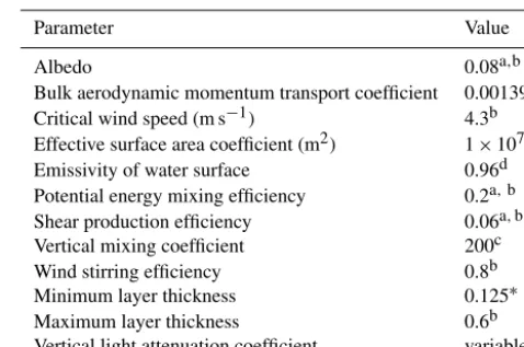
pro-Table 2.DYRESM-WQ-I model parameters. Ice cover parameter can reference Magee et al. (2016) and Magee and Wu (2016).

Parameter Value

Albedo 0.08a,b

Bulk aerodynamic momentum transport coefficient 0.00139b Critical wind speed (m s−1) 4.3b Effective surface area coefficient (m2) 1×107 c Emissivity of water surface 0.96d Potential energy mixing efficiency 0.2a,b Shear production efficiency 0.06a,b,c Vertical mixing coefficient 200c Wind stirring efficiency 0.8b Minimum layer thickness 0.125∗ Maximum layer thickness 0.6b Vertical light attenuation coefficient variablee

∗_{indicates value calibrated in the model. Sources:}a_{Antenucci and Imerito (2003).} b_{Tanentzap et al. (2007).}c_{Yeates and Imberger (2003).}d_{Imberger and}

Patterson (1981).e_{Williams et al. (1980).}

files throughout the year including under ice cover. Secchi depth data for Fish Lake and Lake Wingra were available only from 1995 to the present and collected from the NTL-LTER program. For years with no Secchi data, the long-term mean seasonal Secchi depths were used. There is no signif-icant long-term trend in yearly averaged open-water Secchi depth values for any of the three lakes. Light extinction coef-ficients were estimated from Secchi depth using the equation from Williams et al. (1980):

kd=1.1/z0_s.73, (4)

wherekdis the light extinction coefficient andzsis the Secchi

depth (m).

2.3.4 Meteorological data

the Atmospheric and Oceanic Space Sciences Building in-strumentation tower at the University of Wisconsin-Madison (http://metobs.ssec.wisc.edu/pub/cache/aoss/tower/). Details of this adjustment can be found in Magee et al. (2016) and Hsieh (2012).

2.3.5 Inflow and outflow data

Daily inflow and outflow data for Lake Mendota were obtained and described in detail by Magee et al. (2016). Details of data collection and gap-filling can be found there and are not reproduced for brevity. Inflow and outflow data for Fish Lake and Lake Wingra follow a similar process. Inflow and outflow were estimated as the residual unknown terms of the water budget balancing precipitation, evapo-ration, and lake level. USGS water level data from 1966 to 2003 (http://waterdata.usgs.gov/wi/nwis/dv/?site_no= 05406050&agency_cd=USGS&amp;referred_module=sw) were used to estimate inflow and outflow from surface runoff and groundwater inflow. For early years of simulation, where lake level information was not available, the long-term mean lake level was assumed for calculations. Krohelski et al. (2002) determined that surface runoff accounted for two-thirds of inflowing water while groundwater inflow accounted for one-third of total inflow over the period 1990–1991. Using these values, we attributed two-thirds of the inflowing water as surface runoff using air temperatures to estimate the runoff temperature similar to the method for Lake Mendota in Magee et al. (2016) and one-third of inflowing water as groundwater inflow using an average of groundwater temperature measurements (Hennings and Connelly, 2008). For Lake Wingra, water level was recorded sporadically during the period of interest, and was assumed to be the long-term mean lake level for water budget calculations. As in Fish Lake, Lake Wingra has no surface inflow streams, with inflow values attributed equally to direct precipitation, surface runoff, and groundwater inflow (Kniffin, 2011). Groundwater inflow temperatures were estimated using an average of measurements (Hennings and Connelly, 2008), and surface and direct precipitation were estimated as air temperature.

2.3.6 Observation data

Observation data used for model calibration came from a va-riety of sources. For Lake Mendota, long-term water temper-ature records were collected from Robertson (1989) and the NTL-LTER (2012b). Ice thickness data were gathered from E. Birge, University of Wisconsin (unpublished); D. Lathrop, Wisconsin Department of Natural Resources (unpublished); Stewart (1965); and the NTL-LTER program (2012a). Fre-quency of temperature data varied from one or two profiles per year to several profiles for a given week. Additionally, the vertical resolution of the water profiles varied greatly.

For Fish Lake and Lake Wingra, water temperature data were collected from NTL-LTER only from 1996 to 2014 (2012b). 2.4 Model calibration and evaluation

Model calibration consisted of two processes: (1) closing the water balance to match simulated and observed water lev-els and (2) adjusting the minimum water level thickness to match simulated and observed water temperatures for each lake. Water balance for all three lakes was closed using the method described in Sect. 2.3.5 to match measured water levels to known values and to long-term average water lev-els when elevation information was unknown. Model evap-oration rates were not validated; we assume that evaporative water flux and heat flux were properly parameterized by the model. Model parameters were derived from literature values (Table 2). Within the model, the minimum layer thickness sets the limit for how small a water layer can become before it is merged with the smaller of the layers above or below. If the minimum layer thickness is too large, the model may not have the desired resolution to accurately capture changes in temperature and density that occur over small changes in depth. To calibrate this parameter, the minimum layer thick-ness was varied from 0.05 to 0.5 m in intervals of 0.025 m for the period 1995–2000 for all three lakes, similar to the method in Tanentzap et al. (2007) and Weinburger and Vet-ter (2012). One minimum layer thickness was chosen for all three lakes to keep model formulation and implementation identical among the three lakes, and the final thickness was chosen to be 0.125 m, as it minimized the overall deviation between simulated and observed temperature values for the three lakes.

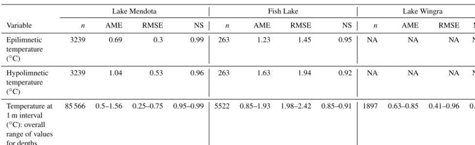
Three statistical measures were used to evaluate model output against observational data (Table 3): absolute mean error (AME), root mean square error (RMSE), and Nash– Sutcliffe (NS) efficiencies were used to compare simulated and observed temperature values for volumetrically aver-aged epilimnion temperature, volumetrically averaver-aged hy-polimnion temperature, and all individual water temperature measurements for unique depth and sampling time combina-tions. Simulated and observed values are compared directly, except for aggregation of water temperature measurements to daily intervals where subdaily intervals are available. Water temperatures were evaluated for the full range of available data on each lake.

2.5 Analysis

Table 3.Absolute mean error (AME), root mean square error (RMSE), and Nash–Sutcliffe efficiency (NS) for water temperature variables on Lake Mendota, Lake Wingra, and Fish Lake.nindicates the number of measurements; NA represents errors that cannot be determined because Lake Wingra is a polymictic lake and does not have an epilimnion or hypolimnion.

Lake Mendota Fish Lake Lake Wingra

Variable n AME RMSE NS n AME RMSE NS n AME RMSE NS

Epilimnetic temperature (◦C)

3239 0.69 0.3 0.99 263 1.23 1.45 0.95 NA NA NA NA

Hypolimnetic temperature (◦_C)

3239 1.04 0.53 0.96 263 1.63 1.94 0.92 NA NA NA NA

Temperature at 1 m interval (◦C): overall range of values for depths

85 566 0.5–1.56 0.25–0.75 0.95–0.99 5522 0.85–1.93 1.98–2.42 0.85–0.91 1897 0.63–0.85 0.41–0.96 0.99

changes in the mean value of lake variables. The variables were tested on data with trends removed using a threshold significance level ofp=0.05, a Huber weight parameter of h=2, and a cut-off length of L=10 years. Coherence of lake variables (Magnuson et al., 1990) for each lake and between lake pairs was determined with a Pearson corre-lation coefficient (Baron and Caine, 2000). The three lakes were paired to compare coherence of lake variables with sur-face area difference (Mendota/Fish pair), depth differences (Fish/Wingra pair), and both surface area and depth differ-ences (Mendota/Wingra). Additionally, temperature, stratifi-cation, and heat flux pair variables for all three lakes are cor-related to air temperature and wind speed drivers, ice date and durations, and temperature, stratification, and heat flux variables within each lake.

To determine the sensitivity of lake water temperature and stratification in response to air temperature and wind speed, we perturbed these drivers across the range of−10 to+10◦C in 1◦C temperature increments and 70 to 130 % of the histor-ical value in 5 % increments, respectively. For each scenario, meteorological inputs remained the same as for the original simulation and snowfall (rainfall) conversion if the air tem-perature scenarios increased (decreased) above 0◦C. Simi-larly, the water balance and water clarity are maintained so that the long-term values in both lakes matches the historical record. This limits our analysis, as it may exclude changes in water temperatures as a result of increased evapotranspira-tion, increased precipitaevapotranspira-tion, or altered water clarity under fu-ture climate scenarios. Inflow temperafu-tures are recalculated for each lake to account for increases or decreases in temper-ature because of air tempertemper-ature changes.

3 Results

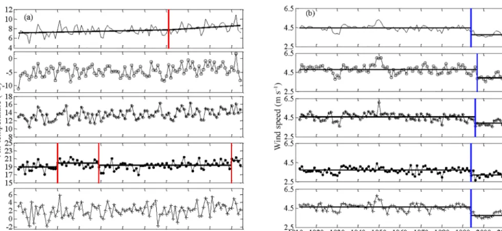
3.1 Changes in air temperature and wind speed Yearly average air temperatures (+0.145◦C decade−1; p< 0.01) and seasonal air temperatures (winter: +0.225◦_{C decade}−1_{; spring +0.165}◦_{C decade}−1_{; summer}

+0.081◦C decade−1; fall +0.110◦C decade−1; p< 0.05) increased from 1911 to 2014 (Fig. 2a). Additionally, yearly average air temperatures, but not seasonal temperatures, showed a significant change in slope occurring in 1981 based on a breakpoint analysis and anF test at a 0.05 significance level (Magee et al., 2016), and summer air temperatures showed three significant abrupt changes in mean value (Fig. 2a). Yearly (−0.073 m s−1decade−1; p< 0.01) and seasonal average (winter: −0.083 m s−1decade−1; spring −0.071 m s−1decade−1; summer: −0.048 m s−1decade−1; fall: −0.088 m s−1decade−1; p< 0.01) wind speeds de-creased from 1911 to 2014 (Fig. 2b). A change in air temperatures also occurred in the 1980s in central Europe (Woolway et al., 2017b), which may indicate that changes in air temperature were a global phenomenon rather than local occurrence. Significant shifts (p< 0.01) in the mean occurred in the mid-1990s for all seasons, but there were no changes in rate of wind speed decreases.

3.2 Model evaluation

Figure 2. Yearly (solid lines), winter (open circles), spring (asterisks), summer (solid circles), and fall (crosses) (a) air temperature and(b)wind speeds for Madison, WI, USA. The red line in the yearly air temperature figure represents a breakpoint in the trend of av-erage air temperature increase from 0.081 to 0.334◦C decade−1occurring in 1981. Red lines in the summer air temperature figure represent abrupt changes in average summer air temperature occurring in 1930, 1949, and 2010. Blue lines in the wind speed figures represent abrupt changes in yearly wind speed change in 1994, winter wind speed in 1997, spring wind speed in 1996, summer wind speed in 1994, and fall wind speed in 1994.

Table 4.Trends and in-lake physical variables for the three studied lakes from 1911 to 2014. Trends are represented as units decade−1. NA indicates data that are not available.

Lake Mendota Fish Lake Lake Wingra

Summer epilimnetic temperature (◦C) +0.069∗∗ +0.138∗ +0.079∗ Summer hypolimnetic temperature (◦C) −0.131∗ −0.083∗ NA Stratification onset (days) 1.15 days earlier∗ 0.81 days earlier∗ NA Fall overturn (days) 1.18 days later∗ 1.05 days later∗ NA Stratification duration (days) +2.68∗ +1.86∗ NA Hypolimnetic heating (◦C) −0.011∗ −0.0011∗ NA Summer Schmidt stability number (J m−2) +11.7∗ +1.44∗ no trend Net shortwave flux (W m−2) no trend no trend no trend Net longwave flux (W m−2) −0.585∗ −0.580∗ −0.459∗ Sensible heat flux (W m−2) +0.410∗ +0.365∗ +0.565∗

Latent heat flux (W m−2) no trend no trend no trend Net heat flux (W m−2) no trend no trend no trend

∗_{indicates significance top< 0.05,}∗∗_{indicates significance top< 0.1 using attest.}

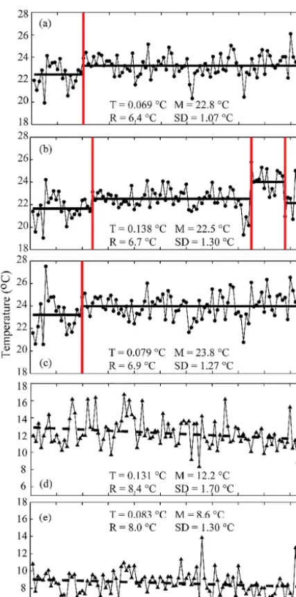
3.3 Summer water temperatures

Lake Mendota and Lake Wingra had similar increasing epil-imnetic water temperature trends, while Fish Lake had a larger increase (Table 4). All three lakes have statistically significant (p< 0.01) abrupt changes in mean epilimnion temperatures over the study period. For Lake Mendota, a change occurs after 1930 from 22.09 to 22.99◦C. For Fish Lake, three changes were detected: after 1934, from 21.68

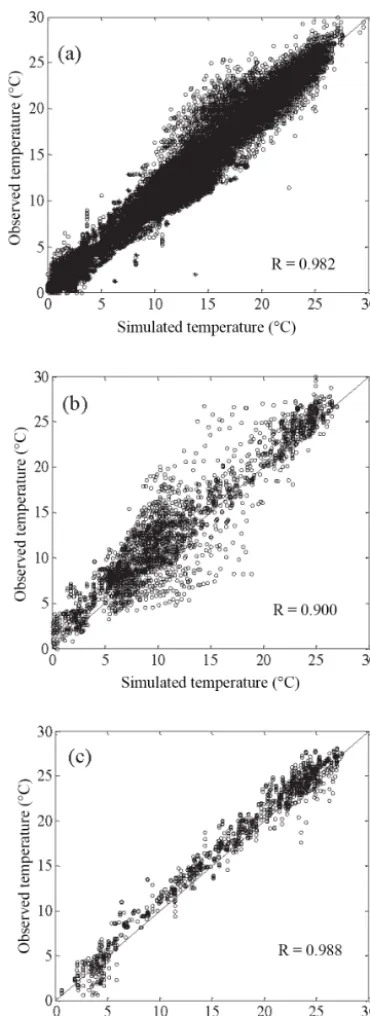
Figure 3.Comparison of observed and simulated water tempera-tures for(a)Lake Mendota,(b)Fish Lake, and(c)Lake Wingra. Each point represents one observation vs. simulation pair with a unique date and lake depth.

temperatures for our study lakes. Additionally, Van Cleave et al. (2014) showed a regime shift in July–September Lake Superior surface water temperatures after 1997, driven by El Niño in 1997–1998; however, we do not find a similar regime shift in our study lakes, which may be due to

geographi-cal differences in meteorology or morphometric differences from the larger Lake Superior.

Lake Mendota and Fish Lake hypolimnions were defined as 20–25 and 13–20 m, respectively, based on the long-term bottom depth of the metalimnion. Lake Mendota has a larger decrease in hypolimnetic temperature than Fish Lake (Ta-ble 4), and neither has an abrupt change in temperature nor a significant breakpoint in linear trend during the study period (Fig. 4). Change in summer (15 July–15 August) hypolim-netic heating was an order of magnitude larger for Mendota than for Fish Lake (Table 4).

3.4 Stratification and stability

We characterize summer stratification by stratification on-set, fall overturn, and duration of stratification (Fig. 5). On-set of stratification and fall turnover were defined as the day when the surface-to-bottom temperature difference was greater than (for stratification) or less than (for overturn) 2◦C (Robertson and Ragotzkie, 1990). Lake Wingra experienced only short-term stratification (timescale of days–weeks) and is excluded from this analysis.

Lake Mendota has larger trend in earlier stratification on-set, fall overturn, and stratification duration than Fish Lake (Table 4), with most of the difference in stratification du-ration caused by larger change in stratification onset date for Lake Mendota. For both lakes, a significant (p< 0.01) shift in onset date occurred at similar times, with a shift to 13.3 days earlier for Lake Mendota after 1994 and 15.1 days earlier for Fish Lake after 1993. No change in trend oc-curred for stratification onset or overturn, but stratification duration shifted from +0.067 to +4.5 days decade−1 _after

1940 for Lake Mendota and from−0.19 days decade−1 _to

+9.6 days decade−1after 1981 for Fish Lake (Fig. 5). We quantify resistance to mechanical mixing with a Schmidt number (Idso, 1973). Lake Mendota showed greater stability in general than Fish Lake (Fig. 6) and had a larger trend of change than Fish Lake (Table 4), possibly due to a larger change in stratification and hypolimnion temperature, increasing stability. There was no significant abrupt shift or change in trend for any of the three lakes during the study period.

3.5 Surface heat fluxes

Figure 4.Mean summertime (15 July–15 August) epilimnetic tem-peratures for (a) Lake Mendota, (b) Fish Lake, and (c) Lake Wingra, and mean summertime (15 July–15 August) hypolimnetic temperatures for (d) Lake Mendota and (e) Fish Lake. In pan-els(a),(b), and(c), solid red lines represent statistically significant (p< 0.05) locations of abrupt changes in epilimnion temperatures and solid lines represent mean temperatures for each period. In pan-els(d)and(e), dashed lines represent the long-term trend over the period 1911–2014.T is the trend of water temperature change per decade,R is the range of temperatures, M is the mean tempera-ture, and SD is the standard deviation in temperatures for the study period. Epilimnion was defined as 0–10 m depth for Mendota, 0– 5 m for Fish, and the whole water column for Wingra based on sur-face mixed layer depth calculated using LakeAnalyzer (Read et al., 2011).

Table 5.Correlation coefficients for lake pairs of simulated open-water lake variables. NA indicates data that are not available.

Lake pair

Lake variable Mendota/ Wingra/ Mendota/ Fish Fish Wingra

Epilimnion temperature 0.601 0.747 0.804 Hypolimnion temperature 0.474 NA NA Stratification onset 0.262 NA NA

Fall overturn 0.388 NA NA

Schmidt stability number 0.827 0.405 0.346 Net shortwave flux 0.995 0.925 0.922 Net longwave flux 0.993 0.969 0.967 Sensible heat flux 0.965 0.887 0.893 Latent heat flux 0.989 0.977 0.984 Net heat flux 0.722 0.630 0.532

than Mendota or Fish, but a larger change in trend for sen-sible heat flux, indicating that depth likely influences the re-sponse of those heat fluxes to air temperature and wind speed changes.

3.6 Coherence between lake pairs

Pearson correlations for all variables and lake pairs are sig-nificant (Table 5). Shortwave, longwave, sensible, and la-tent heat fluxes show high correlation for lake pairs, suggest-ing that morphometry has little impact on variability among lakes. Similarly, epilimnion temperatures have high tempo-ral coherence. However, Fish Lake pairs have lower correla-tions, which may be a result of changes to lake depth (Kro-helski et al., 2002) compared to stable water levels in Men-dota and Wingra. Low coherence between the MenMen-dota/Fish pair for hypolimnion temperature and stratification dates sug-gests that fetch differences impact variability. Stability, how-ever, is lower for pairs with Lake Wingra, indicating that lake depth plays a role in temporal coherence of stability. Sim-ilarly, Lake Wingra pairs have lower coherence of net heat flux although the coherence of heat flux components is rela-tively high. Depth may be influencing a non-linear response of net heat flux that is not present in the components of the flux.

3.7 Correlations between lake variables

Men-Figure 5.Stratification onset (gray) and overturn (black) dates for(a)Lake Mendota and(b)Fish Lake. Stratification duration for(c)Lake Mendota and (d) Fish Lake. Dark circles are modeled results and dashed lines denote the trend line for the 104-year period. In pan-els(a)and(b), dashed lines represent the long-term trend in stratification onset and overturn dates. In panels(c)and(d), solid red lines represent the timing of a statistically significant (p< 0.01) change in trend and solid black lines represent the trend during the periods.Ris the range of onset, overturn, or duration; M is the mean date for onset, overturn, or duration length; and SD is the standard deviation in dates for the study period.

Figure 6.Yearly average summertime (15 July–15 August) Schmidt stability values for Lake Mendota (black) and Fish Lake (gray). Dashed lines represent the long-term trend for each lake.

dota and Fish Lake, but the opposite is true for Lake Wingra, where summer air temperature is not significantly correlated. Additionally, hypolimnion temperature is more highly cor-related with stability in Lake Mendota, whereas epilimnion temperature is more highly correlated with stability in Fish Lake.

3.8 Sensitivity to changes in air temperature and wind speed

Responses of simulated stratification onset, fall overturn, and hypolimnetic temperature to air temperature and wind speed perturbation scenarios for Lake Mendota and Fish Lake are discussed in the following. Other variables are omitted for brevity and Lake Wingra did not experience prolonged strat-ification under any sensitivity scenarios, so they are excluded from the analysis. In our analysis, we refer to the “base case”

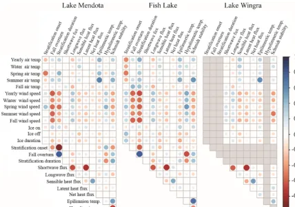
Figure 8.Plots of Pearson correlation coefficients among climate (air temperature and wind speed) variables and lake variables for the three study lakes.

as the meteorological values that represent the historical pe-riod from 1911 to 2014 and refer to perturbations in air tem-perature and wind speed from that base case.

Stratification onset generally occurs earlier on Fish Lake than Lake Mendota for all scenarios (Fig. 9). Simulations show that the response of median onset dates to changes in air temperature is the same for both increases and de-creases from the base case (−2.0 days◦C−1)for Lake Men-dota, but for Fish Lake the magnitude of change is larger for air temperature decreases (−1.5 days◦C−1 for temperature increases and +2.7 days◦C−1 for temperature decreases). Variability in Lake Mendota onset remains consistent across scenarios but decreases for Fish Lake as air temperatures in-crease. This may be from interaction between ice cover and stratification onset on Fish Lake but not on Lake Mendota. For Lake Mendota, stratification onset dates have a larger change for wind speed increases than decreases (−3.4 days (m s−1)−1for decreases and+10.5 days (m s−1)−1for wind speed increases), as is the case for Fish Lake (−3.6 days (m s−1)−1for decreases and+8.1 days (m s−1)−1for wind speed increases). Variability in onset dates decreases with lower wind speeds and increases with higher wind speeds.

Fall overturn typically occurs slightly early on Lake Men-dota than on Fish Lake for all scenarios (Fig. 10). For Lake Mendota, stratification overturn dates change at a rate

of +0.68 days◦_C−1 _{with positive and negative}

perturba-tions in temperature, while Fish Lake has a larger change for air temperature increases (+1.81 days◦C−1 for temper-ature increases and −0.77 days◦C−1 for temperature de-creases) from the historical condition. Standard deviation in overturn dates decreased slightly for Lake Mendota as air temperature increased but remained consistent for Fish Lake. For stratification overturn dates on Lake Mendota, the change is+13.9 days (m s−1)−1 for wind speed decreases and−17.1 days (m s−1)−1for wind speed increases. For Fish Lake, the change is+16.4 days (m s−1)−1for wind speed de-creases and−8.5 days (m s−1)−1for wind speed increases. Like onset dates, variability in overturn dates decreases with lower wind speeds and increases with higher wind speeds.

For both lakes, increases in air temperature increase hy-polimnetic temperatures, while decreases in wind speed decrease temperatures (Fig. 11). Simulations show that the response of median hypolimnetic temperatures to changes in air temperatures is consistent for Lake Men-dota (+0.18◦Chypolimnion C−air temperature1 )for both increases

and decreases from the base case but not so for Fish Lake (+0.25◦Chypolimnion C−air temperature1 for air temperature

in-creases and −0.18◦Chypolimnion C−air temperature1 for air

Figure 9.Day of stratification onset under select air temperature perturbation scenarios for(a)Lake Mendota and(b)Fish Lake and day of stratification onset under select wind speed perturbation scenarios for(c)Lake Mendota and(d)Fish Lake. The box represents the 25th and 75th quartiles and the central line is the median value. The whiskers extend to the minimum and maximum data points in the cases where there are no outliers, which are plotted individually.

Figure 11.Hypolimnetic water temperatures under select air temperature perturbation scenarios for(a)Lake Mendota and(b)Fish Lake and hypolimnetic water temperatures under select wind speed perturbation scenarios for(c)Lake Mendota and(d)Fish Lake. The box represents the 25th and 75th quartiles and the central line is the median value. The whiskers extend to the minimum and maximum data points in the cases where there are no outliers, which are plotted individually.

temperature scenarios remain consistent for both lakes. Hy-polimnion temperatures change inconsistently with increases and decreases in wind speed for both lakes. For Lake Men-dota, the change is −1.1◦_{C (m s}−1₎−1 _{for decreases and}

+1.8◦_{C (m s}−1₎−1_{for wind speed increases. For Fish Lake,}

the change is−1.2◦C (m s−1)−1for decreases and+0.8◦C (m s−1)−1for wind speed increases. Variability decreases for lower wind speeds in Lake Mendota but remains constant for Fish Lake.

4 Discussion

4.1 Model performance and comparison

The DYRESM-WQ-I model reliably simulated water tem-peratures over long-term (1911–2014) simulations (Fig. 3, Table 4). Generally, simulated temperatures were lower than observed values. Some may be attributed to timing of obser-vations, which in most instances occur during midday, when water temperatures may be slightly higher than daily aver-ages, as output from the model. Slight deviation is also ex-pected due to averaging of air temperature and wind speeds. In general, thermocline depths were within 1 m of observed values, but some years differ by as much as 2.5 m, con-tributing additional error in water temperature comparison for depths near the thermocline.

The performance of the DYRESM-WQ-I model was within those of other studies. Perroud et al. (2009)

per-formed a comparison of one-dimensional lake models on Lake Geneva, and RMSEs for water temperatures were as high as 2◦C for the Hostetler model (Hostetler and Bartlein, 1990), 1.7◦_{C for DYRESM (Tanentzap et al., 2007), 2}◦_C

for SIMSTRAT, and 4◦_{C for the Freshwater Lake Model}

(FLake) (Golosov et al., 2007; Kirillin et al., 2012). Similar to this study, errors in the upper layers were lower than those in the bottom of the water column (Perroud et al., 2009). Fang and Stefan (1996) gave standard errors of water tem-perature of 1.37◦C for the open-water season and 1.07◦C for the total simulation period for Thrush Lake, MN, sim-ilar to those here. Nash–Sutcliffe efficiency coefficients for all three study lakes were within the ranges found in Yao et al. (2014) for the Simple Lake Model (SIM; Jöhnk et al., 2008), Hostetler, Minlake (Fang and Stefan, 1996), and Gen-eral Lake Model (GLM; Hipsey et al., 2014) for Harp Lake, Ontario, Canada, water temperatures.

In-flow and outIn-flow measurements were assessed by the USGS for quality assurance and control, but uncertainty for both quantity and water temperature is unknown. The effects of these uncertainties may not be large as the inflow and out-flow are small in comparison to lake volume. The combina-tion of uncertainties in parameters and observed data may be high; however, as all parameters and observational methods were kept consistent among the three lakes, the validity of the model in predicting differences among the three lake types is adequate.

The main limitation in the model and resulting simulations is the assumption of one-dimensionality in both the model and field data. Quantifying the uncertainty from this limita-tion can be difficult (Gal et al., 2014; Tebaldi et al., 2005) Small, stratified lakes generally lack large horizontal temper-ature gradients (Imberger and Patterson, 1981), allowing the assumption of one-dimensionality to be appropriate. How-ever, short-term deviations in water temperature and thermo-cline depth may exist due to internal wave activity, especially in larger lakes (Tanentzap et al., 2007), and spatial variations in wind stress can produce horizontal variations in tempera-ture profiles (Imberger and Parker, 1985). To address the role of internal wave activity and benthic boundary layer mixing, the pseudo two-dimensional deep mixing model by Yeates and Imberger (2003) is employed here. This mixing model has been shown to accurately characterize deep mixing that distributes heat from the epilimnion into the hypolimnion, thus weakening stratification, and the rapid distribution of heat entering the top of the hypolimnion from benthic bound-ary layer mixing, which strengthens stratification (Yeates and Imberger, 2003). Tributary inflows may also contribute to en-hanced diffusion due to inflow momentum; however, lakes used in this study are seepage-dominated lakes with little to no tributary contribution, so this phenomenon does not prevent the one-dimensional model from being applicable in this study. This one-dimensional assumption here and corre-sponding model results may not apply elsewhere for lakes with large inflow volumes.

Additionally, light extinction significantly impacts thermal stratification (Hocking and Straškraba, 1999) and light ex-tinction estimated from Secchi depths can have a large de-gree of measurement uncertainty (Smith and Hoover, 2000), which may result in uncertainty in water temperatures. To address this uncertainty, where available, we use measured Secchi depth values, which have been shown to improve es-timates of the euphotic zone over fixed coefficients (Luhtala and Tolvanen, 2013). Secchi depths were unavailable for por-tions of the simulation period, and average values for the season were used. Analysis comparing using the method of known Secchi depths to both seasonally varying average Sec-chi depths and constant SecSec-chi depths for the lakes indicates that seasonally varying averages do not significantly decrease model reliability when compared to year-specific values but do show improvement over constant Secchi depths.

4.2 Importance of wind speed and other variables

changes than increasing air temperatures for both lakes. This is particularly notable as current research has been dominated by studying air temperature effects and neglecting the role of wind speed changes.

Ultimately, lake warming or cooling may depend on the magnitudes and directions of changes of air temperature, wind speed, and other variables as climatic variables (hu-midity, cloud cover, solar radiation and water clarity) are important in determining lake water temperatures. Schmid and Köster (2016) demonstrated that 40 % of surface wa-ter warming in Lake Zurich was caused by increased solar radiation, and Wilhelm et al. (2006) showed that daily ex-trema of surface equilibrium temperature responded to shifts in wind speed, relative humidity, and cloud cover in addition to changes in air temperature. However, neither study looked at lakes with seasonal ice cover, which may not account for changes in ice sheet formation and the resulting influence on lake water temperatures (Austin and Colman, 2007). Other studies have demonstrated that ice cover changes do not di-rectly influence summer surface water temperatures (Zhong et al., 2016), in agreement with our modeling results (Fig. 8). Changes in underwater light conditions from increased dis-solved organic carbon concentrations combined with reduc-tion in surface wind speeds can result in cooling whole-lake average temperatures despite substantial air tempera-ture increases, as was the case for Clearwater Lake, Canada (Tanentzap et al., 2008). Water clarity has seen both increases and decreases since the early 1990s (Rose et al., 2017), with precipitation playing a critical role in year-to-year variability (Rose et al., 2017). Further investigation into the combined effects of these climatic and lake-specific variables is war-ranted.

4.3 Role of morphometry on water temperature and stratification

4.3.1 Lake depth

Lake depth plays a key role in determining thermal structure and stratification of the three lakes in this study. Even un-der the extreme increases in air temperature, Lake Wingra remained polymictic and did not become dimictic like Lake Mendota or Fish Lake. Additionally, Schmidt stability ex-hibited no trend on the shallow lake, unlike for the deeper two (Table 4). Due to lower heat capacity, shallow lakes re-spond more directly to short-term variations in the weather (Arvola et al., 2009), and heat can be transferred through-out the water column by wind mixing (Nõges et al., 2011). This was particularly evident in correlations among drivers and lake variables, where air temperature did not have a sig-nificant correlation with stability for Lake Wingra, but wind speed was highly correlated. For shallow lakes, wind speed may be a larger driver to temperature structure and stability, with the importance of air temperature increasing with lake depth. Deep lakes have a higher heat capacity so that greater

wind speeds are required to completely mix the lake during the summer months, resulting in more temperature stability and higher Schmidt stability values for deeper Lake Mendota and Fish Lake. Our study is consistent with previous research showing mean lake depths can explain the most variation in stratification trends, and lakes with greater mean depths have larger changes in their stability (Kraemer et al., 2015). Over-all, Lake Wingra had a larger magnitude of latent and net heat fluxes than the deeper lakes. Diurnal variability in surface temperatures is larger for shallow lakes, promoting increased latent heat fluxes in these lakes (Woo, 2007). This increased response may also explain the larger change in trend for sen-sible heat flux since Lake Wingra responds more quickly to changes in air temperature and thus has a larger change in sensible heat flux during each day. Interestingly, net heat flux of Lake Wingra is less coherent with the deeper lakes than the deep lakes are with each other. This may be due to the com-bination of more extreme temperature variability, increasing sensible and latent heat fluxes during the open-water season, and the lower sensitivity of ice cover duration in Lake Wingra compared to the deeper lakes (Magee and Wu, 2017). Ice cover significantly reduces heat fluxes at the surface (Jakkila et al., 2009; Leppäranta et al., 2016; Woo, 2007), and larger changes in ice cover duration for Lake Mendota and Fish Lake compared to Lake Wingra would reduce synchrony of heat fluxes among the three lakes.

4.3.2 Surface area

tempera-ture compared to Fish Lake (Table 5). Additionally, momen-tum from surface stress scales linearly with lake area and non-linearly with wind speed (Yeates and Imberger, 2003; see their Eqs. 31 and 33), making momentum from surface stress, and thus mixing, stratification, and hypolimnion tem-peratures, more variable for lakes with larger fetch and even more variable when wind speed is increased (see Figs. 9–11). Greater variability in momentum and mixing corresponds to larger variability of Schmidt stability for Lake Mendota, with the larger surface area. Greater transfer of momentum in Lake Mendota results in the slightly deeper thermocline for the larger surface area lake (∼10 m in Lake Mendota and ∼6 m in Fish Lake), which may play a role in filter-ing the climate signals into hypolimnion temperatures. Low hypolimnetic temperature coherence between Mendota and Fish suggests that lake morphometry plays a role. This result is consistent with other studies that show lake morphometry parameter affects the way temperature is stored in the lake system (Thompson et al., 2005). Increased momentum on Lake Mendota from the larger surface area may also limit the impact of ice-off dates on stratification onset and hypolim-netic temperatures because the lake has ample momentum to sustain mixing events regardless of ice-off dates, while Fish Lake’s small surface area limits mixing, making ice-off dates and stratification more highly correlated.

5 Conclusion

The combination of increasing air temperatures and decreas-ing wind speeds in Madison-area lakes resulted in warmer epilimnion temperatures, cooler hypolimnion temperatures, longer stratification, increased stability, and greater long-wave and sensible heat fluxes. Increased stratification dura-tions and stability may have lasting impacts on fish popula-tions (Gunn, 2002; Jiang et al., 2012; Sharma et al., 2011), and warmer epilimnion temperatures affect the phytoplank-ton community (Francis et al., 2014; Rice et al., 2015). Shal-low lakes respond more directly to changes in climate, which drives differences in surface heat flux compared to deeper lakes, and wind speed may be a larger driver to temper-ature structure than air tempertemper-atures, with importance of air temperatures increasing as lake depth increases. Larger surface area lakes have greater wind mixing, which influ-ences differinflu-ences in temperatures, stratification, and stability. Climate perturbations indicate that larger lakes have more variability in temperature and stratification variables than smaller lakes, and this variability increases with greater wind speeds. Most significantly, for all three lakes, wind speed plays a role as large as, or larger than, air temperatures in temperature and stratification variables. This reveals that air temperature increases are not the only climate variable that managers should plan for when planning mitigation and adaptation techniques. Previous research has shown uncer-tainty in the changes in hypolimnion water temperatures for

dimictic lakes; however, the perturbation scenarios indicate that while increasing air temperature always increases hy-polimnion temperature, wind speed is a larger driving force, and the ultimate hypolimnion temperature response may be primarily determined by whether the lake experiences an in-crease or dein-crease in wind speeds. Understanding this role in the context of three lakes of differing morphometry is impor-tant when developing a broader understanding of how lakes will respond to changes in climate. Lake water temperatures play a driving role in chemical and biological changes that may occur under future climate scenarios, and identifying differences in this response across lakes will aid in the under-standing of lake ecosystems and provide critical information to guide lake management and adaptation efforts.

Data availability. At last, readers who are interested in ac-cessing the DYRESM code should contact the authors: Chin Wu ([email protected]) or Madeline Magee ([email protected]).

Competing interests. The authors declare that they have no conflict of interest.

Acknowledgements. The authors acknowledge Yi-Fang Hsieh for assisting in the development of an ice module in the DYRESM-WQ model that was originally provided by David Hamilton. We would like to thank Dale Robertson at Wisconsin USGS and Richard (Dick) Lathrop at Center for Limnology for providing valuable long-term observation data for the three study lakes. In addition, we thank John Magnuson at Center of Limnology for his insightful suggestions and valuable comments regarding climate change on lakes. We also thank the editor and anonymous reviewers for providing helpful comments that have greatly improved the manuscript. Research funding was provided in part by the US National Science Foundation Long-Term Ecological Research Program, University of Wisconsin (UW) Water Resources Institute USGS 104(B) Research Project, and the UW Office of Sustain-ability SIRE Award Program. In addition, the first author was funded in part by the College of Engineering Grainer Wisconsin Distinguished Graduate Fellowship.

Edited by: Jan Seibert

Reviewed by: five anonymous referees

References

Antenucci, J. and Imerito, A.: The CWR dynamic reservoir simu-lation model DYRESM, Centre for Water Research, The Univer-sity of Western Australia, 2003.

Arhonditsis, G. B., Brett, M. T., DeGasperi, C. L., and Schindler, D. E.: Effects of Climatic Variability on the Thermal Properties of Lake Washington, Limnol. Oceanogr., 49, 256–270, 2004. Arvola, L., George, G., Livingstone, D. M., Järvinen, M.,

Blenck-ner, T., Dokulil, M. T., Jennings, E., Aonghusa, C. N., Nõges, P., Nõges, T., and Weyhenmeyer, G. A.: The Impact of the Changing Climate on the Thermal Characteristics of Lakes, in: The Impact of Climate Change on European Lakes, edited by: George, G., 85–101, Springer Netherlands, 2009.

Austin, J. A. and Allen, J.: Sensitivity of summer Lake Superior thermal structure to meteorological forcing, Limnol. Oceanogr., 56, 1141–1154, https://doi.org/10.4319/lo.2011.56.3.1141, 2011.

Austin, J. A. and Colman, S. M.: Lake Superior summer water tem-peratures are increasing more rapidly than regional air temper-atures: A positive ice-albedo feedback, Geophys. Res. Lett., 34, L06604, https://doi.org/10.1029/2006GL029021, 2007. Baron, J. and Caine, N.: Temporal coherence of two alpine lake

basins of the Colorado Front Range, USA, Freshw. Biol., 43, 463–476, https://doi.org/10.1046/j.1365-2427.2000.00517.x, 2000.

Birge, E. A., Juday, C., and March, H. W.: The temperature of the bottom deposits of Lake Mendota; a chapter in the heat exchanges of the lake, Trans. Wis. Acad. Sci. Arts Lett., XXIII, available at: http://digicoll.library.wisc.edu/cgi-bin/ WI/WI-idx?type=article&did=WI.WT1927.EABaird&id=WI. WT1927&isize=M (last access: 1 October 2015), 1927. Boehrer, B. and Schultze, M.: Stratification of lakes, Rev. Geophys.,

46, 2006RG000210, https://doi.org/10.1029/2006RG000210, 2008.

Breslow, P. B. and Sailor, D. J.: Vulnerability of wind power resources to climate change in the continental United States, Renew. Energy, 27, 585–598, https://doi.org/10.1016/S0960-1481(01)00110-0, 2002.

Butcher, J. B., Nover, D., Johnson, T. E., and Clark, C. M.: Sensi-tivity of lake thermal and mixing dynamics to climate change, Clim. Change, 129, 295–305, https://doi.org/10.1007/s10584-015-1326-1, 2015.

Carpenter, S. R. and Lathrop, R. C.: Probabilistic Estimate of a Threshold for Eutrophication, Ecosystems, 11, 601–613, https://doi.org/10.1007/s10021-008-9145-0, 2008.

Desai, A. R., Austin, J. A., Bennington, V., and McKinley, G. A.: Stronger winds over a large lake in response to weaken-ing air-to-lake temperature gradient, Nat. Geosci., 2, 855–858, https://doi.org/10.1038/ngeo693, 2009.

Dobiesz, N. E. and Lester, N. P.: Changes in mid-summer water temperature and clarity across the Great Lakes be-tween 1968 and 2002, J. Gt. Lakes Res., 35, 371–384, https://doi.org/10.1016/j.jglr.2009.05.002, 2009.

Fang, X. and Stefan, H. G.: Long-term lake water temperature and ice cover simulations/measurements, Cold Reg. Sci. Technol., 24, 289–304, https://doi.org/10.1016/0165-232X(95)00019-8, 1996.

Ficker, H., Luger, M., and Gassner, H.: From dimictic to monomic-tic: Empirical evidence of thermal regime transitions in three

deep alpine lakes in Austria induced by climate change, Freshw. Biol., 62, 1335–1345, https://doi.org/10.1111/fwb.12946, 2017. Francis, T. B., Wolkovich, E. M., Scheuerell, M. D., Katz, S.

L., Holmes, E. E., and Hampton, S. E.: Shifting Regimes and Changing Interactions in the Lake Washington, USA, Plank-ton Community from 1962–1994, PLoS ONE, 9, e110363, https://doi.org/10.1371/journal.pone.0110363, 2014.

Gal, G., Imberger, J., Zohary, T., Antenucci, J., Anis, A., and Rosen-berg, T.: Simulating the thermal dynamics of Lake Kinneret, Ecol. Model., 162, 69–86, 2003.

Gal, G., Makler-Pick, V., and Shachar, N.: Dealing with uncer-tainty in ecosystem model scenarios: Application of the single-model ensemble approach, Environ. Model. Softw., 61, 360–370, https://doi.org/10.1016/j.envsoft.2014.05.015, 2014.

Gerten, D. and Adrian, R.: Differences in the per-sistency of the North Atlantic Oscillation sig-nal among lakes, Limnol. Oceanogr., 46, 448–455, https://doi.org/10.4319/lo.2001.46.2.0448, 2001.

Golosov, S., Maher, O. A., Schipunova, E., Terzhevik, A., Zdorovennova, G., and Kirillin, G.: Physical background of the development of oxygen depletion in ice-covered lakes, Oecolo-gia, 151, 331–340, https://doi.org/10.1007/s00442-006-0543-8, 2007.

Gunn, J. M.: Impact of the 1998 El Niño event on a Lake Charr, Salvelinus Namaycush, Population Recover-ing from Acidification, Environ. Biol. Fishes, 64, 343–351, https://doi.org/10.1023/A:1016058606770, 2002.

Hadley, K. R., Paterson, A. M., Stainsby, E. A., Michelutti, N., Yao, H., Rusak, J. A., Ingram, R., McConnell, C., and Smol, J. P.: Climate warming alters thermal stability but not stratification phenology in a small north-temperate lake, Hydrol. Process., 28, 6309–6319, https://doi.org/10.1002/hyp.10120, 2014.

Hamilton, D. P. and Schladow, S. G.: Prediction of water quality in lakes and reservoirs. Part I – Model description, Ecol. Model., 96, 91–110, https://doi.org/10.1016/S0304-3800(96)00062-2, 1997. Hamilton, D. P., Magee, M. R., Wu, C. H., and Kratz, T. K.: Ice cover and thermal regime in a dimictic seepage lake under cli-mate change, Inland Waters, in review, 2017.

Hansen, J., Ruedy, R., Sato, M., and Lo, K.: Global sur-face temperature change, Rev. Geophys., 48, RG4004, https://doi.org/10.1029/2010RG000345, 2010.

Hennings, R. G. and Connelly, J. P.: Average ground-water tempera-ture map, Wisconsin, Wisconsin Geological and Natural History Survey, Madison, Wisconsin, USA, 2008.

Hetherington, A. L., Schneider, R. L., Rudstam, L. G., Gal, G., DeGaetano, A. T., and Walter, M. T.: Modeling climate change impacts on the thermal dynamics of polymictic Oneida Lake, New York, United States, Ecol. Model., 300, 1–11, https://doi.org/10.1016/j.ecolmodel.2014.12.018, 2015. Hill, J. M. and Kucera, A.: Freezing a saturated liquid

in-side a sphere, Int. J. Heat Mass Transf., 26, 1631–1637, https://doi.org/10.1016/S0017-9310(83)80083-0, 1983. Hipsey, M. R., Bruce, L. C., and Hamilton, D. P.: GLM – General

Lake Model: Model overview and user information, The Univer-sity of Western Perth, Perth, Australia, 2014.

Holgerson, M. A., Farr, E. R., and Raymond, P. A.: Gas transfer ve-locities in small forested ponds, J. Geophys. Res.-Biogeo., 122, 1011–1021, https://doi.org/10.1002/2016JG003734, 2017. Hostetler, S. W. and Bartlein, P. J.: Simulation of lake evaporation

with application to modeling lake level variations of Harney-Malheur Lake, Oregon, Water Resour. Res., 26, 2603–2612, https://doi.org/10.1029/WR026i010p02603, 1990.

Hsieh, Y.: Modeling ice cover and water temperature of Lake Men-dota, PhD Thesis, University of Wisconsin-Madison, Madison, Wisconsin, USA, 2012.

Idso, S. B.: On the concept of lake stability, Limnol. Oceanogr., 18, 681–683, 1973.

Imberger, J. and Parker, G.: Mixed layer dynamics in a lake exposed to a spatially variable wind field, Limnol. Oceanogr., 30, 473– 488, 1985.

Imberger, J. and Patterson, J. C.: Dynamic reservoir simulation model – DYRESM: 5, in: Transport Models for Inland and Coastal Waters, edited by: Fischer, H. B., 310–361, Academic Press, 1981.

Imberger, J., Loh, I., Hebbert, B., and Patterson, J.: Dynamics of Reservoir of Medium Size, J. Hydraul. Div., 104, 725–743, 1978. Imerito, A.: Dynamic Reservoir Simulation Model DYRESM v4.0 Science Manual, University of Western Australia Centre for Wa-ter Research, 2010.

IPCC: Summary for Policymakers, in: Climate Change 2013: The Physical Science Basis. Contribution of Working Group I to the Fifth Assessment Report of the Intergovernmental Panel on Cli-mate Change, edited by: Stocker, T., Qin, D., Plattner, G.-K., Tig-nor, M., Allen, S. K., Boschung, J., Nauels, A., Xia, Y., Bex, V., and Midgley, P. M., 3–29, Cambridge University Press, Cam-bridge, United Kingdom and New York, NY, USA, 2013. Jakkila, J., Leppäranta, M., Kawamura, T., Shirasawa, K., and

Sa-lonen, K.: Radiation transfer and heat budget during the ice season in Lake Pääjärvi, Finland, Aquat. Ecol., 43, 681–692, https://doi.org/10.1007/s10452-009-9275-2, 2009.

Jiang, L., Fang, X., Stefan, H. G., Jacobson, P. C., and Pereira, D. L.: Oxythermal habitat parameters and identifying cisco refuge lakes in Minnesota under future climate scenarios us-ing variable benchmark periods, Ecol. Model., 232, 14–27, https://doi.org/10.1016/j.ecolmodel.2012.02.014, 2012. Jöhnk, K. D., Huisman, J., Sharples, J., Sommeijer, B., Visser,

P. M., and Stroom, J. M.: Summer heatwaves promote blooms of harmful cyanobacteria, Glob. Change Biol., 14, 495–512, https://doi.org/10.1111/j.1365-2486.2007.01510.x, 2008. Kara, E. L., Hanson, P., Hamilton, D., Hipsey, M. R., McMahon, K.

D., Read, J. S., Winslow, L., Dedrick, J., Rose, K., Carey, C. C., Bertilsson, S., da Motta Marques, D., Beversdorf, L., Miller, T., Wu, C., Hsieh, Y.-F., Gaiser, E., and Kratz, T.: Time-scale depen-dence in numerical simulations: Assessment of physical, chem-ical, and biological predictions in a stratified lake at temporal scales of hours to months, Environ. Model. Softw., 35, 104–121, https://doi.org/10.1016/j.envsoft.2012.02.014, 2012.

Kerimoglu, O. and Rinke, K.: Stratification dynamics in a shal-low reservoir under different hydro-meteorological scenarios and operational strategies, Water Resour. Res., 49, 7518–7527, https://doi.org/10.1002/2013WR013520, 2013.

Kimura, N., Wu, C. H., Hoopes, J. A., and Tai, A.: Diurnal Dy-namics in a Small Shallow Lake under Spatially Nonuniform

Wind and Weak Stratification, J. Hydraul. Eng., 142, 04016047, https://doi.org/10.1061/(ASCE)HY.1943-7900.0001190, 2016. Kirillin, G.: Modeling the impact of global warming on water

tem-perature and seasonal mixing regimes in small temperate lakes, Boreal Environ. Res., 15, 279–293, 2010.

Kirillin, G., Leppäranta, M., Terzhevik, A., Granin, N., Bernhardt, J., Engelhardt, C., Efremova, T., Golosov, S., Palshin, N., Sher-styankin, P., Zdorovennova, G., and Zdorovennov, R.: Physics of seasonally ice-covered lakes: a review, Aquat. Sci., 74, 659–682, https://doi.org/10.1007/s00027-012-0279-y, 2012.

Kniffin, M.: Groundwater status report prepared for Friends of lake Wingra, Edgewood College, Madison, Wisconsin, USA, available at: https://www.lakewingra.org/download/lake_and_ watershed_ecology/groundwaterstatusreport.pdf (last access: 11 November 2016), 2011.

Kraemer, B. M., Anneville, O., Chandra, S., Dix, M., Kuusisto, E., Livingstone, D. M., Rimmer, A., Schladow, S. G., Silow, E., Sitoki, L. M., Tamatamah, R., Vadeboncoeur, Y., and McIntyre, P. B.: Morphometry and average temperature affect lake strat-ification responses to climate change, Geophys. Res. Lett., 42, 4981–4988, https://doi.org/10.1002/2015GL064097, 2015. Krohelski, J. T., Lin, Y.-F., Rose, W. J., and Hunt, R. J.:

Simula-tion of Fish, Mud, and Crystal Lakes and the shallow ground-water system, Dane County, Wisconsin, USGS Numbered Se-ries, U.S. Geological Survey, available at: http://pubs.er.usgs. gov/publication/wri024014 (last access: 24 November 2015), 2002.

Lathrop, R. C., Carpenter, S. R., and Rudstam, L. G.: Water clarity in Lake Mendota since 1900: responses to differing levels of nu-trients and herbivory, Can. J. Fish. Aquat. Sci., 53, 2250–2261, https://doi.org/10.1139/f96-187, 1996.

Leppäranta, M., Lindgren, E., and Shirasawa, K.: The heat budget of Lake Kilpisjärvi in the Arctic tundra, Hydrol. Res., 48, 969– 980, https://doi.org/10.2166/nh.2016.171, 2016.

Livingstone, D. M.: Impact of Secular Climate Change on the Thermal Structure of a Large Temperate Cen-tral European Lake, Clim. Change, 57, 205–225, https://doi.org/10.1023/A:1022119503144, 2003.

Luhtala, H. and Tolvanen, H.: Optimizing the Use of Secchi Depth as a Proxy for Euphotic Depth in Coastal Waters: An Empirical Study from the Baltic Sea, ISPRS Int. J. Geo-Inf., 2, 1153–1168, https://doi.org/10.3390/ijgi2041153, 2013.

Lynch, A. J., Taylor, W. W., Beard Jr., T. D., and Lofgren, B. M.: Climate change projections for lake whitefish (Core-gonus clupeaformis) recruitment in the 1836 Treaty Waters of the Upper Great Lakes, J. Gt. Lakes Res., 41, 415–422, https://doi.org/10.1016/j.jglr.2015.03.015, 2015.

MacIntyre, S. and Melack, J. M.: Mixing dynamics in lakes across climatic zones, in: Lake Ecosystem Ecology: A Global Perspec-tive, edited by: Likens, G. E., 86–95, Academic Press, San Diego, CA, 2010.