Multi decadal analysis of root zone soil moisture applying the exponential filter across CONUS

https://doi.org/10.5194/hess-21-4403-2017 © Author(s) 2017. This work is distributed under the Creative Commons Attribution 3.0 License.

Multi-decadal analysis of root-zone soil moisture applying the

exponential filter across CONUS

Kenneth J. Tobin1, Roberto Torres1, Wade T. Crow2, and Marvin E. Bennett1

1_{Texas A&M International University, Center for Earth and Environmental Studies, Laredo, TX, USA}

2_{United States Department of Agriculture, Agricultural Research Service Hydrology and Remote Sensing Laboratory,} Beltsville, MD, USA

Correspondence to:Kenneth J. Tobin ([email protected])

Received: 1 March 2017 – Discussion started: 11 April 2017

Revised: 6 July 2017 – Accepted: 7 July 2017 – Published: 7 September 2017

Abstract. This study applied the exponential filter to pro-duce an estimate of root-zone soil moisture (RZSM). Four types of microwave-based, surface satellite soil moisture were used. The core remotely sensed data for this study came from NASA’s long-lasting AMSR-E mission. Additionally, three other products were obtained from the European Space Agency Climate Change Initiative (CCI). These datasets were blended based on all available satellite observations (CCI-active, CCI-passive, and CCI-combined). All of these products were 0.25◦and taken daily. We applied the filter to produce a soil moisture index (SWI) that others have suc-cessfully used to estimate RZSM. The only unknown in this approach was the characteristic time of soil moisture varia-tion (T). We examined five different eras (1997–2002; 2002– 2005; 2005–2008; 2008–2011; 2011–2014) that represented periods with different satellite data sensors. SWI values were compared with in situ soil moisture data from the Interna-tional Soil Moisture Network at a depth ranging from 20 to 25 cm. Selected networks included the US Department of En-ergy Atmospheric Radiation Measurement (ARM) program (25 cm), Soil Climate Analysis Network (SCAN; 20.32 cm), SNOwpack TELemetry (SNOTEL; 20.32 cm), and the US Climate Reference Network (USCRN; 20 cm). We selected in situ stations that had reasonable completeness. These datasets were used to filter out periods with freezing temper-atures and rainfall using data from the Parameter elevation Regression on Independent Slopes Model (PRISM). Addi-tionally, we only examined sites where surface and root-zone soil moisture had a reasonably high laggedrvalue (r >0.5). The unknownT value was constrained based on two ap-proaches: optimization of root mean square error (RMSE)

and calculation based on the normalized difference vegeta-tion index (NDVI) value. Both approaches yielded compara-ble results; although, as to be expected, the optimization ap-proach generally outperformed NDVI-based estimates. The best results were noted at stations that had an absolute bias within 10 %. SWI estimates were more impacted by the in situ network than the surface satellite product used to drive the exponential filter. The average Nash–Sutcliffe coeffi-cients (NSs) for ARM ranged from−0.1 to 0.3 and were sim-ilar to the results obtained from the USCRN network (0.2– 0.3). NS values from the SCAN and SNOTEL networks were slightly higher (0.1–0.5). These results indicated that this ap-proach had some skill in providing an estimate of RZSM. In terms of RMSE (in volumetric soil moisture), ARM val-ues actually outperformed those from other networks (0.02– 0.04). SCAN and USCRN RMSE average values ranged from 0.04 to 0.06 and SNOTEL average RMSE values were higher (0.05–0.07). These values were close to 0.04, which is the baseline value for accuracy designated for many satellite soil moisture missions.

1 Introduction

is important also from a water resource standpoint and is a valuable measure in drought monitoring (Bolten et al., 2010; Bolten and Crow, 2012). The dimensions of RZSM also im-pact other systems beyond the hydrologic cycle, most notably with the quantification of carbon fluxes within soils. There-fore, direct sensing of RZSM dynamics will bring us closer to a truer understanding of the carbon soil pool, with obvious implications for future climate change.

Given the importance of RZSM to agricultural and other applications, more effort is needed to understand the im-pacts of climate change associated with this critical vari-able. The National Aeronautics and Space Administration (NASA), European Space Agency (ESA), and other gov-ernments across the world have had a long history of sup-porting missions that generate remotely sensed surface soil moisture, including the Scanning Multichannel Microwave Radiometer (SMMR), the Special Sensor Microwave Imager (SSM/I), Tropical Rainfall Measurement Mission (TRMM), Advanced Microwave Scanning Radiometer-Earth Observ-ing System (AMSR-E), Soil Moisture and Ocean Salinity (SMOS), Soil Moisture Active Passive (SMAP), scatterom-eters on the European remote sensing satellites, which in-cludes scatterometer (SCAT) and the advanced scatterometer (ASCAT) to name only a few (e.g., Lakshmi et al., 1997; Wagner et al., 1999; Kerr et al., 2001; Jackson et al., 2002; Hutchinson, 2003; Njoku et al., 2003; McCabe et al., 2005; Owe et al., 2008; Entekhabi et al., 2010). Passive microwave soil moisture estimates, like AMSR-E-measured horizon-tal and vertical polarization temperatures in several wave-lengths, which include 6.6/6.9 GHz (C band), 10.7 GHz (X band), and 19.3 GHz (Ku band). In addition, the vertical po-larization is examined at 36.5/37.0 GHz (Ka band). An ad-vantage of the more recent SMOS and SMAP missions is that they operate at a lower frequency 1.2/1.4 GHz (L band), which has great penetrative power, especially in highly veg-etated areas. In terms of the active sensors, both SCAT and ASCAT operated at 5.3 GHz (C band) and have a similar de-sign philosophy. These sensors make sequential observations of the backscattering coefficient with six sideways-looking antennas and make sequential observations of the backscat-tering coefficient using three polarizing antennas.

Liu et al. (2012) described the development of two exten-sively validated surface soil moisture products. These prod-ucts were created using a harmonized dataset based on all available soil moisture retrievals: one from the Vienna Uni-versity of Technology (TU Wien) based on active microwave observations (Wagner et al., 2003; Bartalis et al., 2007) and one from the Vrije Universiteit Amsterdam (VUA), in col-laboration with the NASA Goddard Space Flight Center Hy-drological Sciences Laboratory, based on passive microwave observations (Owe et al., 2008). This effort was a part of the ESA Climate Change Initiative (CCI). The harmoniza-tion of these datasets incorporated the advantages of both mi-crowave techniques and spanned the entire period from 1978 onward. This effort is unlike NOAA’s Soil Moisture

Oper-ational Products System (SMOPS), which was a long-term record of soil moisture based on only passive microwave data.

A long-standing goal of the soil remote sensing commu-nity is to develop techniques that can observe changes in RZSM at depths greater than 10 cm, because all of the mis-sions described above are confined to sensing moisture only within the top 5 cm of the profile. In 2015, NASA launched the SMAP mission that had the potential to combine the ad-vantages of passive and active microwave retrievals to es-timate soil moisture dynamics at depth. Unfortunately, early on in this mission, the satellite’s radar failed. Despite this set-back, NASA had invested considerable resources into the de-velopment of an ensemble Kalman filter (EnKF)-based level 4 RZSM product for SMAP (Reichle et al., 2016) and the development of lower-frequency airborne radar systems for deeper penetration of the soil column (via the EV-1 Air-MOSS project). While this work is to be commended, the limited time availability of these products precludes their use for long-term climatic trend studies.

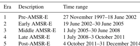
Table 1.Observation eras from 1997 to 2014. Era Description Time range

1 Pre-AMSR-E 27 November 1997–18 June 2002 2 Early AMSR-E 19 June 2002–30 June 2005 3 Middle AMSR-E 1 July 2005–30 June 2008 4 Late AMSR-E 1 July 2008–3 October 2011 5 Post-AMSR-E 4 October 2011–31 December 2014

2 Data

2.1 Era definitions

The data examined in this study span over 17 years. As such, we compared soil moisture produced by the expo-nential filter over five roughly equal eras (3–4.5 years), which were defined based on the available satellite re-trievals during each era (see Liu et al., 2012). These eras included 27 November 1997–18 June 2002 (pre-AMSR-E), 19 June 2002–30 June 2005 (early AMSR-E), 1 July 2005– 30 June 2008 (middle AMSR-E), 1 July 2008–3 Octo-ber 2011 (late AMSR-E), and 4 OctoOcto-ber 2011–31 Decem-ber 2014 (post-AMSR-E; Table 1). The pAMSR-E era re-lied heavily on the TRMM microwave imager (TMI) passive observations and SCAT active retrievals that operated until 2006. In fact, the climatology of the passive dataset during this period was rescaled based on TMI data and likewise the same was true of AMSR-E during eras 2–4. During the early AMSR-E era, passive observations from the WindSat satellite became available online (Gaiser, 2004). The mid-dle AMSR-E era was a time of transition in terms of active observations as the SCAT satellite was replaced by ASCAT. The late AMSR-E era saw the arrival of the ESA SMOS mis-sion. After the failure of AMSR-E, SMOS observations took on a more prominent role within the CCI passive microwave framework. Also during the post-AMSR-E era, the Japanese Space Agency launched AMSR2 (Wentz et al., 2014), which is considered the replacement for the long-lasting AMSR-E mission.

2.2 In situ soil moisture

Direct in situ comparisons were made between RZSM esti-mates with in situ data from the International Soil Moisture Network (ISMN; Dorigo et al., 2011). The ISMN provides access to a host of meteorological and soil moisture data (at many depths). In this study, we selected soil moisture at two depths. Surface soil (0–10 cm) and RZSM (20–25 cm) mois-ture were compared to assess the performance of the expo-nential filter method. In this study, we focused on four net-works within CONUS that have been examined in previous studies. Al Bitar et al. (2012) conducted an extensive evalua-tion of SMOS data using two networks; we utilized the Soil Climate Analysis Network (SCAN; 20.32 cm) and

SNOw-pack TELemetry (SNOTEL; 20.32 cm). Additionally, we ob-tained soil moisture observations from two other CONUS networks: the US Department of Energy Atmospheric Ra-diation Measurement (ARM; 25 cm) program (Jackson et al., 1999) and the US Climate Reference Network (USCRN; 20 cm; Bell et al., 2013). Complete ARM observations only existed from eras 1 to 4, and USCRN data were available for only era 5 (Table 1). In situ values were aggregated to a daily time step (based on UTC time) that matched the sur-face satellite-based soil moisture product described below. Figures 1 and 2 show the location of the stations selected across the five eras.

The ARM network used the Campbell Scientific 229-L heat dissipation matric potential sensor to estimate soil mois-ture (Reece, 1996). Calibration of this method was based on comparison of matric potential with soil water release curves (Klute, 1986). Conversely, the SCAN, SNOTEL, and USCRN networks all used a Stevens Water Hydra Probe (Schaefer et al., 2007; Bell et al., 2013). Seyfried et al. (2005) described the calibration approach and how the dielectric measurements from the Hydra Probe sensor were converted into volumetric soil moisture measurements.

2.3 Surface satellite-based soil moisture

This study was supported by four surface (5 cm) soil mois-ture products, three of which came from the CCI program. We used the CCI-passive, CCI-active, and CCI-combined products (version 2.2). The harmonization process involved in the creation of these products was described by Liu et al. (2012) and these datasets are available online (http://www. esa-soilmoisture-cci.org/node/145). In addition, we also uti-lized stand-alone data from the AMSR-E mission during eras 2–4. In this study, we acquired the version produced by the Land Surface Parameter Model (LPRM; Owe et al., 2008; ftp://hydrol.sci.gsfc.nasa.gov/data/s4pa/WAOB). All of these satellite soil moisture products were produced at a daily time step with a 0.25◦spatial resolution.

2.4 Other datasets

Several other datasets were used in an ancillary role. Air tem-perature and precipitation data were obtained from the Pa-rameter elevation Regression on Independent Slopes Model (PRISM; Daly et al., 1994) from grid cells (4 km spatial res-olution) co-located with examined in situ sites (PRISM Cli-mate Group 2015). These data were used to screen dates be-low freezing and with significant precipitation data, as sug-gested by Dorigo et al. (2011), to enhance quality control.

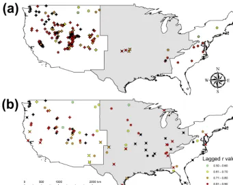
Figure 1.Locality map of examined in situ stations (ARM: X; SCAN:∗; SNOTEL:+) with(a)era 1,(b)era 2, and(c)era 3. The gray area represents the central CONUS, whereas white indicates the eastern and western regions of CONUS.

that were atmospherically corrected to mask water, clouds, aerosols, and cloud shadows. Datasets were provided in a si-nusoidal grid with a 250 m resolution, and an average of nine pixels around each in situ station were used to calculate a global average NDVI for each era.

3 Methods

3.1 Initial station filtering

To ensure selection of the highest-quality in situ stations, we applied two criteria in our initial station selection. The first

Figure 2.Locality map of examined in situ stations (ARM: X; SCAN:∗; SNOTEL:+) with(a)era 4 and(b)era 5. During era 5, X represents USCRN instead of ARM stations. The gray area represents the central CONUS, whereas white indicates the eastern and western regions of CONUS.

laggedrvalue fell below 0.5 were rejected. Qiu et al. (2014) used a similar selection criterion in their study.

3.2 Exponential filter

Wagner et al. (1999) originally developed the exponential fil-ter and Albergel et al. (2008) refined this approach with a more robust recursive version of this method. This version provided an estimate of a soil wetness index (SWI) within the root zone. This index standardized RZSM based on the total range of values recorded by the in situ dataset. The re-cursive formulation provided a predictor of RZSM at time (tn), which in this study was given in days and was derived

as

SWImn=SWImn(n−1)+Kn[ms(tn)−SWImn(n−1)], (1)

where SWImn(n−1)represented the estimated RZSM at time tn−1, ms(tn)was the surface soil moisture estimate based on

either CCI products or AMSR-E retrievals, and Kn was the

gain at timetndetermined with

Kn=

Kn−1

Kn−1+e tn−_tn−1

T

, (2)

whereT represented the timescale of soil moisture variation in days. At the beginning of each era and after excessively

large gaps in ms(tn)data (>12 days), the filter was

initial-ized with SWIm(1)=ms(tn)andKn1set to 1. Results from a data denial experiment described below provided support for the selection of 12 days as an appropriate timescale to reset the filter. The prime advantage of the exponential filter was that the only unknown wasT. Finally, the SWImngenerated

from the exponential filter, which ranged from 0 to 1000, was rescaled to match the range of the in situ data (in volumetric units) allowing for comparisons between these datasets. 3.3 Objective metrics

re-sults are also evaluated based on whether the absolute bias is low (within 10 %) or high (greater than 10 %), which strongly impacts the other objective metrics. Each of these metrics has their own utility as discussed in the paper below.

3.4 Calibration ofTopt

Albergel et al. (2008) noted no significant correlation be-tween soil properties and the optimal timescale of soil mois-ture variation (Topt). Therefore, they constrained this param-eter by optimizing T based on the NS metric, an approach also applied by Ford et al. (2014). However, Albergel et al. (2008) also noted a weak relationship betweenT with cli-mate. Specifically, a linkage between increased temperatures and hence soil evaporation (not transpiration). A lower Topt was representative of a faster response of SWI present in ar-eas with a higher evaporational demand. This conjecture was consistent with a relationship developed by Qiu et al. (2014) using mean NDVI values at in situ sites.

In this study, we used two approaches to determine Topt. The first method optimizedToptat a time in which the RMSE is minimized. This was essentially the same approach as find-ing a maximum NS value. RMSE was calculated between 1 and 68 days at a 1-day increment. Sites that converged on the upper 68-day bound were rejected. Qiu et al. (2014) used a similar upper bound as a means of selecting SCAN sites for their study.

The second approach used the NDVI formulation from Qiu et al. (2014) to calculateTopt. This relationship is given as

Topt= [−75.263×NDVI] +68.171. (3) 3.5 In situ station filtering and data denial experiment To ensure that the exponential filter was effective in produc-ing a RZSM estimate, the ms(tn)term was set based on

sur-face (5 cm) in situ data instead of satellite data. Normally, grid-based satellite surface moisture estimates are used to drive the exponential filter. However, to establish a filter based on the quality of in situ data, an initial estimate of RZSM is determined based on surface in situ data at the 5 cm level. Initial RZSM estimates with a NS value less than 0.50, which is a common threshold for defining a satisfactory match between in situ and simulated hydrologic data (Mori-asi et al., 2007), were rejected. This filter removed many of the poor-performing outliers (NS<−1.00) from considera-tion. Table 2 describes the issues with the remaining poor-performing outliers that lingered after this in situ based fil-tering approach.

Use of surface (5 cm) in situ data also supported a data de-nial experiment that gauged how the filter’s performance was impacted by gaps in the ms(tn)time series. This experiment

focused on the SCAN network during era 3 (2005–2008; Ta-ble 1). Time series were altered to include only data at 2-, 5-, 8-, and 11-day intervals. This experiment was based on the

Table 2.Number of poor-performing (NS<1.00) outliers for all four satellite products.

ARM SCAN SNOTEL USCRN

RMSE optimization

In situ data 17 3 15 1

Insufficient SWI 0 1 14 0

Lack of range 0 11 0 3

Timing issues 0 0 9 0

NDVI approach

In situ data 22 16 32 5

Insufficient SWI 0 3 44 0

Lack of range 0 17 15 8

Timing issues 0 6 5 3

32 out of 42 sites that had in situ based NS in excess of 0.50, i.e., the sites that survived this filtering process. Both surface (5 cm) in situ and satellite (AMSR-E) data were used in this experiment.

3.6 Spurious data filtering

Before calculation of SWI values for all four satellite prod-ucts at each in situ station, a series of filters were applied to remove any spurious results following the quality con-trol guidelines articulated by Dorigo et al. (2013). Surface temperature and precipitation data from co-located PRISM grid cells flagged problematic dates within the time series of each dataset. Satellite retrieval from days in which the minimum air temperature was less than 0◦C were removed from the SWI dataset. Satellite soil moisture retrievals were particularly fraught with difficulty under freezing conditions (Dorigo et al., 2011). Likewise, precipitation can be prob-lematic and days with greater than 1 mm day−1 were ex-cised following the guidance of Dorigo et al. (2013). Three additional flags related to the quality of the in situ data were applied. Days with values in excess of the porosity reported by the ISMN were expunged from the rescaled SWI dataset. Likewise, days that recorded the same value (plateaus) or zero were deemed spurious and removed. The final filtered rescaled SWI dataset consisted of less than 100 days; this dataset was rejected following the guidance of Dorigo et al. (2013). Finally, SWI based estimates in which NS<−1.00 were rejected as outliers. A detailed discussion of these outliers is given below.

4 Results

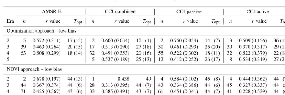
iden-Table 3.Average laggedrvalues andToptbetween SWI based and in situ soil moisture at the 25 cm depth for the ARM network. Standard derivation is indicated in parentheses. Thenvalue represents the number of observations.

AMSR-E CCI-combined CCI-passive CCI-active

Era n rvalue Topt n rvalue Topt n rvalue Topt n rvalue Topt

Optimization approach – low bias

1 – – – 14 0.471 (0.249) 30 (19) 4 0.614 (0.131) 25 (29) 9 0.450 (0.193) 26 (13)

2 9 0.587 (0.080) 4 (1) 10 0.491 (0.136) 9 (4) 10 0.554 (0.103) 7 (6) 11 0.493 (0.153) 17 (7)

3 12 0.589 (0.148) 7 (3) 12 0.520 (0.156) 12 (10) 12 0.615 (0.165) 8 (4) 12 0.460 (0.165) 13 (10)

4 4 0.666 (0.053) 32 (10) 3 0.707 (0.081) 10 (4) 2 0.649 (0.011) 12 (1) 1 0.823 5

NDVI approach – low bias

1 – – – 17 0.439 (0.241) 36 (3) 9 0.480 (0.171) 36 (2) 12 0.414 (0.172) 36 (4)

2 7 0.622 (0.156) 35 (3) 11 0.567 (0.172) 34 (4) 9 0.642 (0.132) 34 (4) 13 0.484 (0.154) 32 (3)

3 13 0.559 (0.204) 34 (2) 12 0.437 (0.179) 35 (3) 10 0.645 (0.137) 34 (3) 12 0.341 (0.197) 34 (3)

4 5 0.666 (0.053) 32 (6) 3 0.704 (0.004) 34 (2) 3 0.665 (0.542) 34 (2 7 0.323 (0.184) 32 (3)

1 2 5 8 11

-0.5 0 0.5 1

NS

Intervals (days)

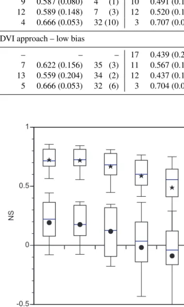
Figure 3.Box plot of the data denial experiment from the SCAN network during era 3 (2005–2008). Results for day 1 represent base-line data for the exponential filter driven by surface soil moisture data (in situ data:F; low absolute bias RMSE-optimized AMSR-E:•). Other time series were altered to include only data at 2-, 5-, 8-, and 11-day intervals.

tical to the results based on in situ surface soil moisture datasets in which every other day was withheld. Even in datasets with every four out of five dates withheld there was only a slight drop in performance. This result underscored the ability of the exponential filter to effectively cope with datasets that have significant gaps. Average NS values fell to 0.5 only when over 90 % of the surface soil moisture dataset was withheld and measurements from only every 11th day were used. The data denial experiment using AMSR-E data to drive the filter yielded a similar drop-off in performance as the number of withheld days increased.

Figures 1 and 2 show laggedrvalues between in situ sur-face (5 cm) and RZSM (20–30 cm) during the five eras. ARM sites clustered in Oklahoma and Kansas had higher lagged rvalues during era 1 (network averager=0.864) and a drop in this metric during eras 2 to 4 (network averager=0.793– 0.796). SCAN sites exhibited correlation coefficients that varied spatially. In general, better performances were noted from eastern (network averager=0.751–0.872) and central sites (network averager=0.812–0.874). Western sites had slightly lowerr values (network averager=0.699–0.770). Notable outliers were present for the stations in Montana during eras 4 and 5 (Fig. 2) that could account partly for the poorer performance noted during these eras. SNOTEL stations were concentrated in the western CONUS and had consistently high correlation coefficients (network average r=0.828–0.865). Finally, the USCRN sites examined dur-ing era 5 (Table 1) generally had betterr values in eastern and central CONUS (network averager=0.846–0.882) as opposed to the west (network averager=0.768).

The remainder of this section focuses on the results from the exponential filter driven by the four satellite products. TheToptand laggedrvalues discussed are based on results that have a low absolute bias (±10 %). Note that the propor-tion of sites that recorded low bias varies between networks (data not shown). Most ARM stations were characterized by having low bias (76–100 %), whereas SNOTEL sites had the lowest number of sites with a low bias (32–45 %). SCAN (53–60 %) and USCRN (60–66 %) had an intermediate num-ber of sites with a low bias. The subsequent results focused only on the low bias stations.

Table 4.Average laggedrvalues andToptbetween SWI based on optimization and in situ soil moisture at the 20.32 cm depth for the SCAN network (Figs. 1 and 2). Standard derivation is indicated in parentheses. Thenvalue represents the number of observations.

AMSR-E CCI-combined CCI-passive CCI-active

Era n rvalue Topt n rvalue Topt n rvalue Topt n rvalue Topt

Optimization approach – low bias

1 – – – 1 0.817 19 1 0.691 1 3 0.458 (0.323) 22 (10)

2 4 0.691 (0.157) 39 (19) 7 0.598 (0.157) 27 (16) 2 0.661 (0.007) 16 (9) 7 0.519 (0.147) 15 (6)

3 17 0.596 (0.129) 10 (7) 19 0.556 (0.164) 14 (13) 16 0.556 (0.184) 9 (5) 17 0.521 (0.140) 17 (17) 4 14 0.697 (0.096) 15 (14) 16 0.698 (0.155) 19 (15) 10 0.720 (0.176) 15 (12) 16 0.642 (0.226) 17 (16)

5 – – – 17 0.572 (0.183) 16 (15) 11 0.472 (0.192) 21 (14) 15 0.589 (0.195) 14 (14)

NDVI approach – low bias

1 – – – 2 0.678 (0.199) 32 (6) 2 0.747 (0.096) 49 4 0.463 (0.282) 40 (10)

2 6 0.554 (0.198) 34 (16) 7 0.541 (0.179) 30 (12) 1 0.330 20 10 0.505 (0.171) 28 (7)

3 14 0.596 (0.111) 31 (10) 15 0.480 (0.193) 34 (11) 15 0.613 (0.095) 36 (11) 15 0.471 (0.187) 31 (10) 4 16 0.573 (0.242) 37 (15) 20 0.585 (0.223) 39 (15) 14 0.615 (0.238) 39 (15) 20 0.608 (0.226) 40 (15)

5 – – – 19 0.518 (0.220) 39 (13) 15 0.428 (0.238) 46 (11) 26 0.469 (0.237) 41 (13)

Table 5.Average laggedr values andToptbetween SWI based on optimization and in situ soil moisture at the 20.32 cm depth for the SNOTEL network. Standard derivation is indicated in parentheses. Thenvalue represents the number of observations.

AMSR-E CCI-combined CCI-passive CCI-active

Era n rvalue Topt n rvalue Topt n rvalue Topt n rvalue Topt

Optimization approach – low bias

2 5 0.572 (0.311) 17 (15) 2 0.600 (0.034) 10 (1) 2 0.750 (0.054) 14 (7) 3 0.509 (0.156) 36 (13)

3 39 0.463 (0.264) 20 (15) 17 0.513 (0.290) 27 (18) 30 0.461 (0.293) 25 (20) 30 0.370 (0.317) 29 (11) 4 63 0.508 (0.299) 18 (14) 32 0.491 (0.353) 20 (16) 55 0.522 (0.302) 18 (11) 32 0.522 (0.379) 22 (18)

5 – – – 5 0.527 (0.189) 25 (13) 12 0.412 (0.252) 26 (17) 8 0.534 (0.319) 27 (21)

NDVI approach – low bias

2 2 0.678 (0.197) 44 (13) 1 0.438 49 4 0.584 (0.102) 45 (8) 4 0.444 (0.362) 44 (7)

3 44 0.367 (0.374) 44 (6) 28 0.313 (0.395) 44 (7) 43 0.334 (0.386) 44 (6) 45 0.327 (0.337) 44 (5) 4 71 0.425 (0.367) 43 (6) 33 0.385 (0.491) 43 (7) 61 0.451 (0.341) 44 (7) 41 0.228 (0.529) 44 (6)

5 – – – 11 0.425 (0.216) 44 (7) 9 0.357 (0.318) 43 (5) 10 0.590 (0.268) 42 (6)

range of average era Topt (28–46 days; Table 3). However, again, optimization produced more variable Toptvalues (9– 39 days; Table 4). A similar pattern was noted at SNOTEL sites. The NDVI approach yielded higher network average eraToptvalues (42–45 days) vs. the more variable and lower results from the optimization method (17–36 days; Table 5). Finally, USCRN sites from era 5 (Table 1) exhibited a broad range of values for both approaches (NDVI of 30–55 days; optimization of 9–28 days; Table 6).

Tables 3–6 show results from the direct correlation be-tween in situ RZSM- and SWI-based estimates generated from the four satellite products. Network average values are excluded in this discussion if there were less than three mea-surements within an era for a network. Generally, but not al-ways, the optimization approach yielded higher laggedr val-ues than NDVI. Interestingly, in the ARM network, in 5 out of 14 instances, the NDVI approach yielded network

aver-ager values that were greater than those obtained from the optimization method (Table 3). ARM sites from the central Great Plains had network averager values based on opti-mization that ranged from 0.450 to 0.707 across eras 1–4 (Table 1), whereas the NDVI approach yielded a lower and broader variation inrvalues (0.323–0.704; Table 3).

Table 6.Average laggedr valuesToptbetween SWI based on optimization and in situ soil moisture at the 20 cm depth for the USCRN network during era 5. Standard derivation is indicated in parentheses. Sites are divided by region (east, central, west) as indicated in Fig. 2. Thenvalue represents the number of observations.

CCI-combined CCI-passive CCI-active

Region n rvalue Topt n rvalue Topt n rvalue Topt

Optimization approach – low bias

East 1 0.105 4 – – – 1 0.486 15

Central 13 0.594 (0.185) 9 (8) 6 0.707 (0.086) 17 (19) 11 0.607 (0.126) 6 (3)

West 1 0.857 11 4 0.406 (0.125) 28 (21) 3 0.540 (0.389) 9 (1)

NDVI approach – low bias

East 2 0.388 (0.122) 1 1 0.071 25 2 0.410 (0.133) 21

Central 12 0.521 (0.231) 30 (10) 7 0.605 (0.194) 35 (9) 7 0.534 (0.176) 25 (7) West 3 0.209 (0.068) 36 (20) 4 0.342 (0.128) 45 (20) 3 0.087 (0.122) 55 (5)

Era 1 Era 2 Era 3 Era 4 Era 5 Era 1 Era 2 Era 3 Era 4 Era 5

AMSR-E CCI-combined CCI-passive CCI-active -0.8 -0.6 -0.4 -0.2 0 0.2 0.4 0.6 0.8 1 -0.8 -0.6 -0.4 -0.2 0 0.2 0.4 0.6 0.8 1 NS NS -1 -0.8 -0.6 -0.4 -0.2 0 0.2 0.4 0.6 0.8 -1 -0.8 -0.6 -0.4 -0.2 0 0.2 0.4 0.6 0.8

Figure 4.Box plots that depict the NS metric for the ARM (eras 1– 4) and USCRN (era 5) networks. Results for high absolute bias optimized datasets are squares, low absolute bias RMSE-optimized datasets are circles, and low absolute bias NDVI datasets are triangles.

SNOTEL stations from the intermountain west showed the greatest variability. Some sites recordedrvalues below 0, but there were also quite a few sites with high correlation coeffi-cients (>0.75). However, in general, network averager val-ues were lower in SNOTEL (optimization of 0.370–0.572; NDVI of 0.228–0.590) than at SCAN western sites (Table 5). Finally, the data from USCRN sites during era 5 (Table 1) had higher network averager values in central sites vs. the western CONUS (Table 6).

NS values across the five eras were depicted in Figs. 4–6. Stations with low absolute bias (±10 %) consistently

outper-Era 1 Era 2 Era 3 Era 4 Era 5 Era 1 Era 2 Era 3 Era 4 Era 5

AMSR-E CCI-combined CCI-passive CCI-active -0.8 -0.6 -0.4 -0.2 0 0.2 0.4 0.6 0.8 1 -0.8 -0.6 -0.4 -0.2 0 0.2 0.4 0.6 0.8 1 NS NS -1 -0.8 -0.6 -0.4 -0.2 0 0.2 0.4 0.6 0.8 -1 -0.8 -0.6 -0.4 -0.2 0 0.2 0.4 0.6 0.8

Figure 5.Box plots depicting the NS metric for the SCAN network. Symbols are the same as in Fig. 4.

Era 1 Era 2 Era 3 Era 4 Era 5 Era 1 Era 2 Era 3 Era 4 Era 5 AMSR-E CCI-combined CCI-passive CCI-active -0.8 -0.6 -0.4 -0.2 0 0.2 0.4 0.6 0.8 1 -0.8 -0.6 -0.4 -0.2 0 0.2 0.4 0.6 0.8 1 NS NS -1 -0.8 -0.6 -0.4 -0.2 0 0.2 0.4 0.6 0.8 -1 -0.8 -0.6 -0.4 -0.2 0 0.2 0.4 0.6 0.8

Figure 6.Box plots depicting the NS metric for the SNOTEL net-work. Symbols are the same as in Fig. 4.

Era 1 Era 2 Era 3 Era 4 Era 5 Era 1 Era 2 Era 3 Era 4 Era 5

AMSR-E CCI-combined CCI-passive CCI-active 0.04 0.08 0.12 0.16 0.04 0.08 0.12 0.16 RMSE RMSE 0 0.04 0.08 0.12 0 0.04 0.08 0.12

Figure 7. Box plots depicting the RMSE metric for the ARM (eras 1–4) and USCRN (era 5) networks. Symbols are the same as in Fig. 4.

Figures 7–9 depicted RMSE values again across the five eras (Table 1). In many respects, RMSE mirrors NS as a per-formance metric. Like NS stations, RMSE values with a low absolute bias outperformed those with high bias. However, the difference between low and high bias datasets was gen-erally not as pronounced for the RMSE metric as it was for NS. However, like with NS, RMSE results showed no dis-cernable temporal trends. RMSE values from the ARM and USCRN networks were illustrated in Fig. 7. Network average

Era 1 Era 2 Era 3 Era 4 Era 5 Era 1 Era 2 Era 3 Era 4 Era 5

AMSR-E CCI-combined CCI-passive CCI-active 0.04 0.08 0.12 0.16 0.04 0.08 0.12 0.16 RMSE RMSE 0 0.04 0.08 0.12 0 0.04 0.08 0.12

Figure 8.Box plots depicting the RMSE metric for the SCAN net-work. Symbols are the same as in Fig. 4.

Era 1 Era 2 Era 3 Era 4 Era 5 Era 1 Era 2 Era 3 Era 4 Era 5

AMSR-E CCI-combined CCI-passive CCI-active 0.04 0.08 0.12 0.16 0.04 0.08 0.12 0.16 RMSE RMSE 0 0.04 0.08 0.12 0 0.04 0.08 0.12

Figure 9.Box plots depicting the RMSE metric for the SNOTEL network. Symbols are the same as in Fig. 4.

Figure 10.Selected time series associated with poorly performing (NS<1.00) outliers with in situ data as solid gray and SWI estimates in dashed black. Panel(a)shows an example of problematic in situ data. Panel(b)is an example where there was insufficient SWI data. Panel

(c)illustrates an SWI dataset that lacked the dynamic range present in the in situ data. Panel(d)depicts a discrepancy in timing between SWI and in situ datasets. Dates are indicated in mm/dd/yyyy format.

5 Discussion and conclusions

A long-standing goal of the soil remote sensing community has been to develop techniques that can observe changes in RZSM. Regrettably, the technology had not yet progressed to support a global RZSM product based only on remote sens-ing retrievals. The use of land surface models such as the community NOAH model (Chen et al., 1996), Global Land Data Assimilation System (GLDAS; Rodell et al., 2007), and European Centre for Medium-Range Weather Forecasts (ECMWF) reanalysis products (Uppala et al., 2005; Massari et al., 2014) have been used to fill this gap in recent years. These platforms have become popular and provide an esti-mate of root-zone soil moisture that has been applied to field-scale studies (Albergel et al., 2012; Blankenship et al., 2016; Kedzior and Zawadski, 2016). In addition, another approach that has been suggested is based on thermal infrared-based remote sensing (e.g., Hain et al., 2011).

Besides ease of use, the exponential filter methodology is an attractive alternative because it leverages existing

re-jected as not suitable. At these sites, perhaps the fundamental assumption of the exponential filter method that there was hydrologic equilibrium between the surface and root zone was violated. Therefore, the gross errors recorded at some sites cannot be ascribed to issues with the exponential filter, and the data denial experiment demonstrated the robustness of this method at least in certain instances (Fig. 3).

Extending this approach, we examined the quality of ex-ponential filter results driven by surface in situ data against background conditions including soil texture, land cover, and climate zone (data not shown). In terms of soil texture, in situ sites with loamy textures has a general tendency to out-perform (based on NS value) sand- or clay-dominated sites. This is not surprising given that the exponential filter gener-ally works best when soil moisture is moderate (Ford et al., 2014). Soil textures with a low available water capacity such as sand and clay are more likely to have extreme, both dry and wet, moisture contents. In terms of land cover, the only consistent result is that in the SNOTEL network the more open rangeland settings exhibited slightly better NS values than forest-dominated areas. However, this pattern was not observed at sites from the other networks. Finally, there is no clear trend in performance of the exponential filter as a function of climate zone.

Analysis of poor-performing outliers (NS<−1.00) pro-vided additional insights into how the exponential filter can fail at some sites (Table 2). Within the ARM network, all outliers could be attributed to in situ data issues such as spikes, breaks, anomalous high values that exceed soil poros-ity, anomalous low values at zero, and extended plateaus (Dorigo et al., 2013). An example of such a clearly flawed in situ dataset is shown in Fig. 10a. Within the SNOTEL net-work, there was more of a mix in error type (Table 3). Besides in situ data issues, another significant source of error was the limited number of days in some of the final SWI datasets. Following the guidance of Dorigo et al. (2010), SWI datasets with less than 100 days were rejected. However, based on observations in this study, significant issues of representa-tiveness were noted when there were less than 400 days (Fig. 10b). The high altitude of many SNOTEL sites resulted in a longer freezing season during which a greater number of days were filtered out. There were some sites with in situ data issues in the SCAN network (Table 2). However, many of the outliers also were caused by either SWI values that lacked the dynamic range of the in situ dataset (Fig. 10c) or SWI val-ues that had significant timing offsets compared with in situ RZSM observations (Fig. 10d). These issues were the result of either site non-representativeness or errors in surface soil moisture retrievals. Finally, USCRN sites exhibited a similar mix of errors as noted in the SCAN network (Table 2).

A consistent result noted in this study was the impact of bias on other performance metrics. Consistently better re-sults for all metrics were noted (Tables 3–6; Figs. 4–9) when there was a low absolute bias (within 10 %) vs. SWI datasets that had a high absolute bias (>10 %). Additionally, this

ob-servation was observed for SWI values produced with both approaches to constrainT (minimization of RMSE and the NDVI approach). The impact of bias on standard objective metrics was a focus of temporal stability analysis (Vachaud et al., 1985; Martinez-Fernandez and Ceballos, 2005). Sites with little variation in bias yielded more robust comparisons with remote sensing data (Starks et al., 2006), which is a re-sult that was confirmed in this study across four distinct in situ soil moisture networks and satellite products.

Interestingly, the results observed in this study were more impacted by the in situ network than the surface satellite product used to drive the exponential filter. In terms of the NS metric, SCAN, SNOTEL, and USCRN outperformed ARM (Figs. 4–6). The NS metric seemed to have a greater utility in identifying outliers than the RMSE metric. This was because it ranged from 1.00 to potentially−∞, unlike RMSE, which ranged in this study from only 0 to 0.14.

Conversely, when considering the RMSE metric, ARM sites yielded superior scores compared with SCAN, SNO-TEL, and USCRN (Figs. 7–9). Within the ARM network av-erage RMSE was less than 0.04, which is the baseline value for accuracy designed for many satellite soil moisture mis-sions (e.g., Kerr et al., 2001; Entekhabi et al., 2010). SCAN and USCRN were slightly above this guideline and were similar to RMSE values noted in previous in situ/satellite soil moisture comparisons (e.g., Brocca et al., 2010; Jack-son et al., 2010, 2012; Al Bitar et al., 2012). According to the RMSE metric, SNOTEL sites performed the worst and was significantly above the 0.04 performance target.

Perhaps the most interesting result from this study was that the performance metrics in each in situ network did not vary over time. Given that almost two decades of data were examined, this finding is particularly noteworthy. Therefore, SWI estimates of RZSM produced by the exponential filter using CCI datasets can be leveraged for long-term, perhaps even multi-decadal, climate studies (Manfreda et al., 2011). Another fruitful line of future research could compare ex-ponential filter estimates of RZSM with those generated by land surface models. With the proliferation of space-based remote sensing platforms and the continued development of in situ monitoring networks, the duration of RZSM time se-ries will only grow. As such, the approaches outlined in this work can provide the cornerstone to support future assess-ments of long-term trends in RZSM, which is an essential climate variable.

Data availability. The harmonization process involved in the cre-ation of the surface soil moisture products was described by Liu et al. (2012), and these datasets are available online (http://www. esa-soilmoisture-cci.org/node/145).

Competing interests. The authors declare that they have no conflict of interest.

Acknowledgements. We acknowledge the support of the NASA

Climate Indicator and Data Products for the National Climate Assessments program through award no. NNX16AH30G. The assistance of Robert Parinussa (University of New South Wales), Arturo Diaz (Texas A&M International University), and Luis Carrasco Garza (Texas A&M International University) is greatly appreciated.

Edited by: Erwin Zehe

Reviewed by: two anonymous referees

References

Albergel, C., Rüdiger, C., Pellarin, T., Calvet, J.-C., Fritz, N., Frois-sard, F., Suquia, D., Petitpa, A., Piguet, B., and Martin, E.: From near-surface to root-zone soil moisture using an exponential fil-ter: an assessment of the method based on in-situ observations and model simulations, Hydrol. Earth Syst. Sci., 12, 1323–1337, https://doi.org/10.5194/hess-12-1323-2008, 2008.

Albergel, C., de Rosnay, P., Balsamo, G., Isaksen, L., and Munoz-Sabater, J.: Soil moisture analyses at ECMWF: evaluation using global-based in situ observations, Remote Sens. Environ., 118, 215–226, 2012.

Al Bitar, A., Leroux, D., Kerr, Y. H., Merlin, O., Richaume, P., Sa-hoo, A., and Wood, E. F.: Evaluation of SMOS soil moisture products over Continental US using the SCAN/SNOTEL Net-work, IEEE T. Geosci. Remote, 50, 1572–1586, 2012.

Bartalis, Z., Wagner, W., Naeimi, V., Hasenauer, S., Sci-pai, K., Bonekmap, H., Figa, J., and Anderson, C.: Initial soil moisture retrievals from the METOP-A Advanced Scat-terometer (ASCAT), Hydrol. Land Surf. Stud., 34, L02401, https://doi.org/10.1029/2007GL031088, 2007.

Bell, J. E., Palecki, M. A., Baker, C. B., Collins, W. G., Lawrimore, J. H., Leeper, R. D., Hall, M. E., Kochendorfer, J., Meyers, T. P., Wilson, T., and Diamond, H. J.: US Climate Reference Network soil moisture and temperature observations, J. Hydrometeorol., 14, 977–988, 2013.

Blankenship, C. B., Case J. L., Zavodsky, B. T., and Crosson, W. L.: Assimilation of SMOS retrievals in the Land Information Sys-tem, IEEE T. Geosci. Remote, 54, 6320–6332, 2016.

Bolten, J. D. and Crow, W. T.: Improved prediction of quasi-global vegetation conditions using remotely-sensed surface soil moisture, Geophys. Res. Lett., 39, L19406, https://doi.org/10.1029/2012GL053470, 2012.

Bolten, J. D., Crow, W. T., Zhan, X., Jackson, T. J., and Reynolds, C. A.: Evaluating the utility of remotely sensed soil moisture re-trievals for operational agricultural drought monitoring, IEEE J. Sel. Top. Appl., 3, 57–66, 2010.

Brocca, L., Morbidelli, R., Melone, F., and Moramarco, T.: Soil moisture spatial variability in experimental areas of central italy, J. Hydrol., 333, 356–373, 2007.

Brocca, L., Melone, F., Moramarco, T., Wagner, W., Naeimi, V., Bartalis, Z., and Hasenauer, S.: Improving runoff pre-diction through the assimilation of the ASCAT soil

mois-ture product, Hydrol. Earth Syst. Sci., 14, 1881–1893, https://doi.org/10.5194/hess-14-1881-2010, 2010.

Chen, F., Mitchell, K., Schakke, J., Xue, Y., Pan, H., Koren, V., Duan, Y., Ek, M., and Betts, A.: Modeling of land-surface evapo-ration by four schemes and comparison with FIFE Observations, J. Geophys. Res., 101, 7251–7268, 1996.

Crow, W. T., Berg, A. A., Cosh, M. H., Loew, A., Mohanty, B. P., Panciera, R., de Rosnav, P., Ryu, D., and Walker, J. P.: Upscal-ing sparse ground -based soil moisture observations for the vali-dation of course-resolution satellite soil moisture products, Rev. Geophys., 50, 2011RG000372, 2012.

Daly, C., Neilson, R. P., and Phillips, D. L.: A statistical-topographic model for mapping climatological precipitation over mountainous terrain, J. Appl. Meteorol., 33, 140–158, 1994. Dorigo, W. A., Scipal, K., Parinussa, R. M., Liu, Y. Y., Wagner, W.,

de Jeu, R. A. M., and Naeimi, V.: Error characterisation of global active and passive microwave soil moisture datasets, Hydrol. Earth Syst. Sci., 14, 2605–2616, https://doi.org/10.5194/hess-14-2605-2010, 2010.

Dorigo, W. A., Wagner, W., Hohensinn, R., Hahn, S., Paulik, C., Xaver, A., Gruber, A., Drusch, M., Mecklenburg, S., van Oeve-len, P., Robock, A., and Jackson, T.: The International Soil Mois-ture Network: a data hosting facility for global in situ soil mois-ture measurements, Hydrol. Earth Syst. Sci., 15, 1675–1698, https://doi.org/10.5194/hess-15-1675-2011, 2011.

Dorigo, W. A., Xavier, A., Vreugdenhill, M., Gruber, A., Hegyiová, A., Sanchis-Dufau, A. D., Zamojski, D., Cordes, C., Wag-ner, W., and Drusch, M.: Global automated quality con-trol of in situ soil moisture data from the International Soil Moisture Network, Vadose Zone J., 12, vzj2012.0097, https://doi.org/10.2136/vzj2012.0097, 2013.

Entekhabi, D., Njoku, E. G., O’Neill, P. E., Kellogg, K. H., Crow, W. T., Edelstein, W.N., Entin, J. K., Goodman, S. D., Jackson, T. J., Johnson, J., Kimball, J., Piepmeir, J. R., Koster, R. D., Martin, N., McDonald, K. C., Moghaddam, M., Moran, S., Reichle, R., Shi, J. C., Spencer, M. W., Thurman, S. W., Tsnag, L., and Van Zyl, J.: The Soil Moisture Active Passive (SMAP) mission, P. IEEE, 98, 704–716, 2010.

Ford, T. W., Harris, E., and Quiring, S. M.: Estimating root zone soil moisture using near-surface observations from SMOS, Hy-drol. Earth Syst. Sci., 18, 139–154, https://doi.org/10.5194/hess-18-139-2014, 2014.

Gaiser, P. W., St. Germain, K. M., Twarog, E. M., Poe, G. A., Purdy, W., Grossman, W., Jones, W. L. Spencer, D., Golba, G., Cleveland, J., Choy, L., and Bevilacqua, R. M.: The WindSat spaceborne polarimetric microwave radiometer: Sensor descrip-tion and early orbit performance, IEEE T. Geosci. Remote, 42, 2347–2361, 2004.

Hain, C. R., Crow, W. T., Mecikalski, J. R. Anderson, M. C., and Holmes, T.: An intercomparison of available soil moisture estimates from thermal-infrared and passive mi-crowave remote sensing, J. Geophys. Res.-Atmos., 166, D15107, https://doi.org/10.1029/2011JD015633, 2011.

Hutchinson, J. M. S.: Estimating near-surface soil moisture using active microwave satellite imagery and optical sensor inputs, T. ASAE, 46, 225–236, 2003.

South-ern Great Plains Hydrological Experiment, IEEE T. Geosci. Re-mote, 37, 2136–2151, 1999.

Jackson, T. J., Hsu, A. Y., and O’Neill, P. E.: Surface soil moisture retrieval and mapping using high-frequency microwave satellite observations in the Southern Great Plains, J. Hydrometeorol., 3, 688–699, 2002.

Jackson, T. J., Cosh, M. H., Bindlish, R., Starks, P. J., Bosch, D. D., Seyfried, M., Goodrich D. C., Moran, M. S., and Du, J.: Valida-tion of Advanced Microwave Scanning Radiometer Soil Mois-ture Products, IEEE T. Geosci. Remote, 48, 4256–4272, 2010. Jackson, T. J., Bindlish, R., Cosh, M. H., Zhoa, T., Starks, P. J.,

Bosch, D. D., Seyfried, M., Moran, M. S., Goodrich, D. C., Kerr, Y. H., and Leroux, D.: Validation of Soil Moisture and Ocean Salinity (SMOS) Soil Moisture Over Watershed Networks in the US, IEEE T. Geosci. Remote, 50, 1530–1543, 2012.

Kedzior, M. and Zawadski, J.: Comparative study of soil moisture from SMOS satellite mission, GLDAS database, and cosmic ray-neutrons measurements at COSMOS in Eastern Poland, Geo-derma, 283, 21–31, 2016.

Kerr, Y. H., Waldteufel, P., Wigneron, J. P., Maerinuzzi, J. M., Font, J., and Berger, M.: Soil moisture retrieval from space: The Soil Moisture and Ocean Salinity (SMOS) mission, IEEE T. Geosci. Remote, 39, 1729–1735, 2001.

Klute, A.: Water retention: Laboratory methods, Methods of Soil Analysis: Part 1, in: Physical and Minerological Methods, edited by: Klute, A., American Society of Agronomy and Soil Science Society of America, 635–662, 1986.

Kumar, S. V., Reichle, R. H., Koster, R. D., Crow, W. T., and Peters-Lidard, C. D.: Role of subsurface physics in the assimilation of surface soil moisture observations, J. Hydrometeorol., 10, 1534– 1547, 2009.

Lakshmi, V., Wood, E. F., and Choudhury, B. J.: Investigation of effect of heterogeneities in vegetation and rainfall on simulated SSM/I brightness tempeatures, J. Appl. Meteorol., 36, 1309– 1328, 1997.

Lettenmaier, D. P., Alsdorf, D., Dozier, J., Huffman, G. J., Pan, M., and Wood, E. F.: Inroads of remote sensing into hydrologic sci-ence during the WRR era, Water Resour. Res., 51, 7309–7342, 2015.

Liu, Y. Y., Dorigo, W. A., Parinussa, R. M., de Jeu, R. A. M., Wag-ner, W., McCabe, M. F., Evans, J. P., and van Dijk, A. I. J. M.: Trend-preserving blending of passive and active microwave soil moisture retrievals, Remote Sens. Environ., 123, 280–297, 2012. Manfreda, S., Lacava, T., Onorati, B., Pergola, N., Di Leo, M., Margiotta, M. R., and Tramutoli, V.: On the use of AMSU-based products for the description of soil water con-tent at basin scale, Hydrol. Earth Syst. Sci., 15, 2839–2852, https://doi.org/10.5194/hess-15-2839-2011, 2011.

Manfreda, S., Brocca, L., Moramarco, T., Melone, F., and Sheffield, J.: A physically based approach for the estimation of root-zone soil moisture from surface measurements, Hydrol. Earth Syst. Sci., 18, 1199–1212, https://doi.org/10.5194/hess-18-1199-2014, 2014.

Martinez-Fernandez, J. and Ceballos, A.: Mean soil moisture esti-mation using temporal stability Analysis, J. Hydrol., 312, 28–38, 2005.

Massari, C., Brocca, L., Barbetta, S., Papathanasiou, C., Mimikou, M., and Moramarco, T.: Using globally available soil moisture indicators for flood modelling in Mediterranean catchments,

Hy-drol. Earth Syst. Sci., 18, 839–853, https://doi.org/10.5194/hess-18-839-2014, 2014.

McCabe, M. F., Gao, H., and Wood, E. F.: Evaluation of AMSR-E-derived soil moisture retrievals using ground-based and PSR air-borne data using SMEX02, J. Hydrometeorol., 6, 864–877, 2005. Moriasi, D. N., Arnold, J. G., Van Liew, M. W., Bingner, R. L., Harmel, R. D., and Veith, T. L.: Model evaluation guidelines for systematic quantification of accuracy in watershed simulations, T. ASABE, 50, 885–900, 2007.

Njoku, E. G., Jackson, T. J., Lakshmi, V., Chan, T. K., and Nghiem, S. V.: Soil moisture retrieval from AMSR-E, IEEE T. Geosci. Remote Sens., 41, 215–229, 2003.

Owe, M., De Jeu, R. A. M., and Holmes, T. R. H.: Multi-sensor historical climatology of satellite-derived global land surface moisture, J. Geophys. Res.-Earth, 113, F01002, https://doi.org/10.1029/2007JF000769, 2008.

Peterson, A. M., Helgason, W. D., and Ireson, A. M.: Esti-mating field-scale root zone soil moisture using the cosmic-ray neutron probe, Hydrol. Earth Syst. Sci., 20, 1373–1385, https://doi.org/10.5194/hess-20-1373-2016, 2016.

Qiu, J., Crow, W. T., Nearing, G. S., Mo, X., and Liu, S.: The impact of vertical measurement depth on the information content of soil moisture time series data, Geophys. Res. Lett., 41, 4997–5004, 2014.

Reece, C. F.: Evaluation of a line heat dissipation sensor for measur-ing soil matric potential, Soil Sci. Soc. Am. J., 60, 1022–1028, 1996.

Reichle, R., De Lannoy, G., Koster, R., Crow, W., and Kimball, J.: SMAP L4 9 km EASE-Grid Surface and Root Zone Soil Mois-ture Geophysical Data, Version 2, NASA National Snow and Ice Data Center, 2016.

Rodell, M., Houser, P. R., Jambor, U., Gottschalck, J., Mitchell, K., Meng, C.-J., Arsenault, K., Cosgrove, R., Schaefer, G. L., Cosh, M. H., and Jackson, T. J.: The USDA Natural Resources Con-servation Service Soil Climate Analysis Network (SCAN), J. At-mos. Ocean. Tech., 24, 2073–2077, 2007.

Schaefer, G. L., Cosh, M. H., and Jackson, T. J.: The USDA Natural Resources Conservation Service Soil Climate Analysis Network (SCAN), J. Atmos. Ocean. Tech., 24, 2073–2077, 2007. Seyfried, M. S., Grant, L. E., Du, E., and Humes, K.: Dielectric

loss and calibration of the Hydra Probe soil water sensor, Vadose Zone J., 4, 1070–1079, 2005.

Starks, P. J., Heathman, G. C., Jackson, T. J., and Cosh, M. H.: Tem-poral stability of soil moisture profile, J. Hydrol., 324, 400–411, 2006.

Tucker, C. J.: Red and photographic infrared linear combinations for monitoring vegetation, Remote Sens. Environ., 8, 127–150, 1979.

Vachaud, G., DeSilnas, A. P., Balabanis, P., Vauclin, M.: Tempo-ral stability of spatially measured soil water probability density function, J. Soil Sci. Soc. Am., 49, 822–828, 1985.

Wagner, W, Lemoine, G, and Rott, H.: A method for estimating soil moisture from ERS scatterometer and soil data, Remote Sens. Environ., 70, 191–207, 1999.

Wagner, W., Scipal, K., Pathe, C., Gerten, D., Lucht, W., and Rudolf, B.: Evaluation of the agreement between the first global remotely sensed soil moisture data with model and precipitation data, J. Geophys. Res.-Atmos., 108, 4611, https://doi.org/10.1029/2003JD003663, 2003.

Wentz, F. J., Meissner, T., Gentemann, C., Hilburn, K. A., and Scott, J.: Remote sensing systems GCOM-W1 AMSR2 Environmental Suite on 0.25 deg grid, Remote Sensing Systems, Santa Rosa, Calfornia, USA, 2014.

Western, A. W., Zhou, S. L., Grayson, R. B., McMahon, T. A., Bloschl, G., and Wilson, D. J.: Spatial correlation of soil mois-ture in small catchments and its relationship to dominant spatial hydrological processes, J. Hydrol., 286, 113–134, 2004. Wilson, D. J., Western, A. W., and Grayson, R. B.: Identifying