Geostatistical interpolation by quantile kriging

https://doi.org/10.5194/hess-23-1633-2019 © Author(s) 2019. This work is distributed under the Creative Commons Attribution 4.0 License.

Geostatistical interpolation by quantile kriging

Henning Lebrenz1,2and András Bárdossy2

1_{University of Applied Sciences and Arts – Northwestern Switzerland, Institute of Civil Engineering, Muttenz, Switzerland} 2_{University of Stuttgart, Institute for Modelling Hydraulic and Environmental Systems, Stuttgart, Germany}

Correspondence:Henning Lebrenz ([email protected]) Received: 18 May 2018 – Discussion started: 30 May 2018

Revised: 1 March 2019 – Accepted: 5 March 2019 – Published: 20 March 2019

Abstract. The widely applied geostatistical interpolation methods of ordinary kriging (OK) or external drift kriging (EDK) interpolate the variable of interest to the unknown lo-cation, providing a linear estimator and an estimation vari-ance as measure of uncertainty. The methods implicitly pose the assumption of Gaussianity on the observations, which is not given for many variables. The resulting “best linear and unbiased estimator” from the subsequent interpolation optimizes the mean error over many realizations for the en-tire spatial domain and, therefore, allows a systematic under-(over-)estimation of the variable in regions of relatively high (low) observations. In case of a variable with observed time series, the spatial marginal distributions are estimated sepa-rately for one time step after the other, and the errors from the interpolations might accumulate over time in regions of relatively extreme observations.

Therefore, we propose the interpolation method of quan-tile kriging (QK) with a two-step procedure prior to in-terpolation: we firstly estimate distributions of the variable over time at the observation locations and then estimate the marginal distributions over space for every given time step. For this purpose, a distribution function is selected and fit-ted to the observed time series at every observation loca-tion, thus converting the variable into quantiles and defin-ing parameters. At a given time step, the quantiles from all observation locations are then transformed into a Gaussian-distributed variable by a 2-fold quantile–quantile transfor-mation with the beta- and normal-distribution function. The spatio-temporal description of the proposed method accom-modates skewed marginal distributions and resolves the spa-tial non-stationarity of the original variable. The Gaussian-distributed variable and the distribution parameters are now interpolated by OK and EDK. At the unknown location, the resulting outcomes are reconverted back into the estimator

and the estimation variance of the original variable. As a summary, QK newly incorporates information from the tem-poral axis for its spatial marginal distribution and subsequent interpolation and, therefore, could be interpreted as a space– time version of probability kriging.

In this study, QK is applied for the variable of observed monthly precipitation from raingauges in South Africa. The estimators and estimation variances from the interpolation are compared to the respective outcomes from OK and EDK. The cross-validations show that QK improves the estimator and the estimation variance for most of the selected objective functions. QK further enables the reduction of the temporal bias at locations of extreme observations. The performance of QK, however, declines when many zero-value observa-tions are present in the input data. It is further revealed that QK relates the magnitude of its estimator with the magnitude of the respective estimation variance as opposed to the tradi-tional methods of OK and EDK, whose estimation variances do only depend on the spatial configuration of the observa-tion locaobserva-tions and the model settings.

1 Introduction

eron, 1965) is given as

E[Z(x)] =m(x)=const., (1)

VAR[Z(x+h)−Z(x)] =2γ (h), (2) in whichγ (h)is the semi-variogram. The incrementZ(x+

h)−Z(x)is assumed as a stationary random function and its variance only depends on the translation vectorh. The set of outcomes by the interpolation to the unknown locationx is described by the linear estimatorZ∗(x)as a measure of their centrality and by the estimation (or kriging) varianceσ_K2(x)

as a measure of the associated uncertainty.

The stated hypothesis entails three implications: the first condition of the intrinsic hypothesis (Eq. 1) demands the variable to be spatially stationary and yields an unbiased estimation error in the entire domain (Chilès and Delfiner, 1999). Therefore, a systematic under-(over-)estimation is in-duced for regions of high (low) observations. Secondly, the marginal distribution of the observed data should ideally be Gaussian in order to be adequately described. Unfortunately, the distribution often departs from the ideal case (Journal and Alabert, 1989), necessitating an a priori transformation of the marginal distribution. And last, the second condition (Eq. 2) implies that the magnitude of the kriging varianceσ_K2(x)only depends on the spatial configuration of the observation lo-cations, the a priori variance of all observations and on the selected variogram model, but not on the magnitude of the linear estimatorZ∗(x)itself (Goovaerts, 2000).

The theoretical extension of external drift kriging (EDK, Ahmed and deMarsily, 1987) addresses the first implication. EDK can be attributed to the non-stationary geostatistical in-terpolation methods and has been frequently applied in var-ious disciplines of practice and science (e.g., Bourennane et al., 2000, van de Kassteele et al., 2009, Motaghian and Mohammadi, 2011). It incorporates additional information from external variables (or drifts) Yj(x)for the estimation of the variable at the unknown location. The meanm(x)is non-stationary but linearly depends on the external variables. Thus, the first condition (Eq. 1) is reformulated to

E[Z(x)]=a+ k X

i=1

bi·Yi((x)), (3)

where k is the number of the incorporated external drifts

Yi(x), whilea,bi are the unknown constants. The drifts are

E[I (x;zth)]=m=const. (4)

This nonlinear transformation is relatively robust and limits the effect of high values on the description of the variable at the unknown location. However, a loss of information comes along by the transformation into a binary variable. Therefore, probability kriging defines multiple thresholds and uses the order relation of the observed variable (Carr and Mao, 1993), being implemented by using co-kriging in the derived multi-variate context. Both non-parametric methods have been sub-ject to research, especially for detection limit problems of groundwater contamination (e.g., Goovaerts et al., 2005; Lee et al., 2007; Adhikary et al., 2011).

In summary, geostatistical methods have been derived in the past in order to address the stated shortfalls of the intrin-sic hypothesis. However, all present methods only regard the observations from the one respective time step for the estima-tion of their marginal spatial distribuestima-tion, but do not incorpo-rate observations from other time steps. The inclusion of a temporal behavior into the geostatistical models is mostly ir-relevant for the original geological variables. However, the temporal variability of a variable becomes more prominent for other sciences, e.g., hydrology, where observations from raingauges over several time steps are implemented into the geostatistical models in order to generate spatial precipitation estimates. These estimates subsequently serve as input to the hydrological modeling (e.g., Syed et al., 2003; Basistha et al., 2008; Cole and Moore, 2008) over multiple time steps. As-sociated errors in the precipitation estimates may ultimately lead to greater errors in the subsequent discharge modeling (Kobold and Sušelj, 2005). These errors strongly depend on the spatial and temporal distribution of the input precipitation (Gabellani et al., 2007; Moulin et al., 2009) and may limit the accuracy of rainfall–runoff simulations. There are geostatis-tical space–time models in order to incorporate the temporal variability of the variable, but they are primarily aiming on the extrapolation of the variable in time (Snepvangers et al., 2003). Therefore, they require a strong dependence of the variable over time, suited, e.g., for groundwater modeling where temporal changes occur relative slowly. This temporal dependence might be absent for other variables, e.g., monthly precipitation.

distributions over space and the independence of the error distribution from the magnitude of the observation.

2 Materials and methods

The theory of quantile kriging (QK) is outlined along with the major theoretical implications, followed by a general dis-cussion of the underlying geostatistical model and a case study for the variable of monthly precipitation is presented.

A preliminary analysis of the selected variable exemplary reveals (Fig. 1) the non-Gaussianity within the data and that the first assumption of the intrinsic hypothesis (see Eq. 1) is not fulfilled since, e.g.,Et[Z(x57, t )] 6=Et[Z(x29, t )]. 2.1 Theory of quantile kriging

QK presumes the existence of observations of the variable

z over consecutive time stepst (=1,2, . . ., J )at every ob-servation locationxi =(x1i, x2i)(for the two-dimensional spaceR2), providing an observed time seriesz(xi, t )at every observation locationi (=1,2, . . ., ni). QK proceeds first with a two-step procedure prior to interpolation (see Sect. 2.1.1) and second with the interpolation itself (see Sect. 2.1.2). 2.1.1 Estimation of the temporal and the spatial

marginal distribution

At first, the distribution over time is estimated at every obser-vation location locationxi: an appropriate theoretical cumu-lative distribution function (cdf)F is selected and fitted to the corresponding time series of observations z(xi, t ), yielding nispecific distributionsF (z(xi, t )). The distributions are de-fined by their corresponding parameter sets2(xi)(=ϑk(xi) withk=1,2, . . ., K) of theK-parametric distribution func-tionF. The quantilesw(xi, t )(=F (z(xi, t );2(xi)) are cal-culated from the observed values of the variablez(xi, t )and the defining parameter set2(xi). The quantilesw(xi, t ) pos-sess a uniform distribution over time on the interval[0,1]for a given observation locationxi. However, their empirical dis-tribution in space is not uniform on[0,1]. In order to profit from the optimality of kriging, it requires a transformation into a Gaussian distribution as a prerequisite of the subse-quent interpolation.

The marginal spatial distribution corresponding to a time step t is, therefore, estimated by a 2-fold quantile–quantile conversion as the second step: the two-parametric beta dis-tribution is fitted to the quantiles w(xi, t ) of a given time stept, whose cdfG(w;α, β)is defined as

G(w;α, β)= α+β−1

X

n=α

(5)

_(α+β−1)! n! ·(α+β−1−n)!·w

n_·(1−w)(α+β−1−n)

on the interval[0,1]by the two parametersα >0 andβ >0. The quantilesG(w(xi, t );α(t ), β(t ))from Eq. (5) are finally transformed by a normal score transformation into the stan-dard Gaussian variable u(xi, t ) with Nu[0|1], which ulti-mately serves as spatial marginal distribution to the subse-quent geostatistical interpolation.

The transformation via the quantiles into the variableu ac-counts for spatially non-stationary distributions of the orig-inal variablezwithE[Z(x, t )] 6=mand exchanges the two conditions of Eqs. (1) and (2) to

E[Fx(Z(x, t ))] =m=const., (6)

VAR[Fx+h(Z(x+h, t ))−Fx(Z(x, t ))] =2γ (h), (7) resolving the problem of spatial non-stationarity. QK can accommodate skewed marginal distributions of the original variable Z, which is similar to probability kriging, but it newly incorporates the temporal behavior ofZ into its es-timation of the spatial marginal distribution.

2.1.2 Interpolation to the unknown location

The outlined conversion of the variablez(xi, t )into the vari-ableu(xi, t )and its corresponding parameter set2(xi) en-tails separate interpolations to the unknown locationx.

The inherent assumption of second-order stationarity im-plies the existence of a constant spatial mean for the variable

uwithin the domain for every time stept. The transformed quantiles are implicitly assumed to be more homogeneously distributed over space than the original variablez. The vari-ableu is subject to a stationary geostatistical interpolation method (e.g., OK), providing a linear estimatorU∗(x, t )and the estimation varianceσ_K,U2 (x, t ). They jointly describe the Gaussian distribution of the random variable U (x, t ) with

N[U∗|σ_K,U2 ].

The defining parameters ϑk (for k=1,2, . . ., K) of the K-parametric distribution functionF are independent from the time step t and they are separately interpolated to the unknown location x. The separate interpolation, however, requires the independence of the parametersϑk from each other. Therefore, a principal component analysis examines the “observed” parameters ϑk(xi)in the Cartesian coordi-nate system (ϑ1|ϑ2|. . .|ϑK) and determines the correspond-ing rotation angleαand translation vectork. The coordinate system is then rotated and translated accordingly prior to in-terpolation in order to ensure independence. A possible spa-tial non-stationarity of the parameters can be accounted for by the choice of an appropriate non-stationary interpolation method (e.g., EDK). The interpolation of the independent pa-rameters yields their estimators at the unknown locationx, which are rotated and translated back to the original coor-dinate system. Thus, the estimatorsϑ_k∗(x)are defining the distribution function at the unknown locationx.

Figure 1. Histogram from the times series of observed monthly precipitation for two random stations: “Laingsnek”, x₅₇ with z=

81.3 mm(a)and “Tambotieboom”,x29withz=38.3 mm(b).

(Sect. 2.1.1), but in reverse order: first the distribution of the quantilesG(W (x, t );α, β)of the beta distribution is calcu-lated by the inverse of the normal score transformation. The distribution of the quantilesW (x, t )are calculated next using the inverse of Eq. (5) and last, the distribution of the original variableZ(x, t )is estimated by using the inverse of the se-lected cdf, being defined by the estimators of its parameters

ϑ_k∗(x). The reconversion of the distribution ofU (x, t )to the distribution ofZ(x, t )can be implemented by the simple nu-merical Rosenblueth point estimation method (Rosenblueth, 1975). The resulting distribution of the original variable Z

is then described by the expectation valueZ∗(x, t )and the varianceσ_K2(x, t ). Note that the resulting asymmetrical dis-tribution of Z(x, t ) is non-Gaussian due to the conversion with the nonlinear but monotonic theoretical cdfF.

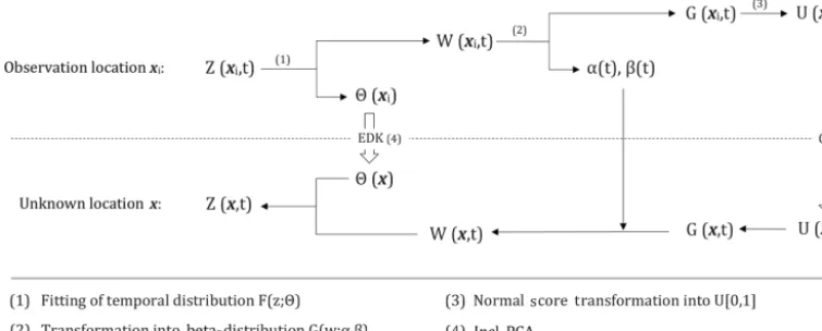
The basic methodology of the proposed QK is illustrated in Fig. 2.

2.2 Discussion of the geostatistical model

Since the proposed method of QK is applied for the variable of monthly precipitation (see Sect. 2.3), the discussion of the underlying process model is based on the following proper-ties of precipitation fields:

– The monthly (and even daily) precipitation amounts

z(x, t ) for a given time step t often show a skewed distribution and cannot be considered as stationary over space. The differences in expected precipitation amounts become especially obvious for long time ac-cumulations.

– The meteorological processes, which are generating precipitation, are usually of large spatial extent: if one location receives heavy precipitation, it is likely that other locations also receive heavy precipitation. – Correlations between time series of precipitation

indi-cate a strong spatial dependence, while the spatial de-pendence of precipitation at one given time step (e.g., day, month) usually show a much weaker spatial depen-dence.

A possible process model reflecting the above properties can be described as follows.

LetU (x, t )be independent (for each different time stept) normal stationary spatial fields withE[U] =0 andD2(U )=

1 for each time stept. Now, the processM(t )is introduced in order to reflect large-scale meteorological processes. High

M(t )values correspond to heavy precipitation covering the area, while low values correspond to dry conditions, as it is reflected by seasonal variations of precipitation amounts. The introducedMmodifies the spatial process to

G(x, t )=U (x, t )+M(t ), (8)

where M(t ) is a process (only in time) with a mean of zero. We may assume that the distribution ofM(t )is normal and, therefore,G(x, t ) would be normally distributed with

N (0, d)(withd= q

1+σ_M2) at every locationx.

For each individual time stept, the distribution ofG(x, t )

isN (M(t ),1)and the resulting spatial fieldW is the tempo-ral non-exceedance probability at locationx being confined to 0≤W (x, t )≤1 and formally described as

W (x, t )=80,d(G(x, t )), (9)

where80,dis the distribution function ofN (0, d). The pre-cipitation is then generated as

Z(x, t )=F_x−1(W (x, t )), (10)

whereFx is the distribution function of precipitation at the locationx. The distribution functionsFx may vary between different locationsx due to topography and other influenc-ing factors, and they could be subject to interpolation (e.g., Mosthaf and Bárdossy, 2017).

We useW (x, t )for each time steptand assume that it fol-lows a beta distribution. In fact, its distribution depends on

M(t ). IfM(t )=0 for all time stepst, then monthly precipi-tation can be fully characterized by independent realizations over space. In this case, the distribution ofW is uniform for eacht.

Figure 2.Flowchart for the basic methodology of quantile kriging.

domain. This is controlled byM(t ), which can be taken, e.g., as an independent random variable or to follow an ARMA process. If M(t )6=0 then the distribution ofW (x, t )is not uniform for this specific time step t. The exact form of the corresponding distribution would be something like

Gt(v)=80,1

8−_{M(t ),}1 ₁(v). (11)

However, the use of Eq. (11) would require the estimation of

M(t ) for each time stept. We decided to use a simple beta distribution instead. The reason for assuming a beta distri-bution is due to their flexibility and their ability to describe distributions well within the interval[0,1].

The introduction ofM(t )is reasonable as it explains the difference between the correlation between stations and the spatial correlation calculated using a variogram type ap-proach for a given time step. The later correlations are usu-ally lower (smaller ranges), which are increased by the com-mon large-scale weather described by M(t ). Note that the introduction of M(t )leads to a correlation of the precipita-tion time series even if the individual snapshots ofU (x, t )

are independent in space.

We estimate and subsequently interpolate Fx within the proposed methodology by the preceding conversion of the variableZ(x_i, t ). In addition, we calculateW (x_i, t )for the observation locations xi and interpolate it to the unknown location x in order to come back to Z(x, t ). In here, spa-tial variograms are calculated for W for each time step t, assuming W to be spatially stationary. Non-Gaussian and non-stationary distributions only occur for the precipitation amounts (i.e., the variableZ).

Non-Gaussianity should be considered due to the usually skewed distribution of precipitation amounts and it only ap-plies to the marginal distribution at a given time stept. The suggested model should enable a simulation of the precipi-tation amounts. The spatial dependencies are considered to correspond to a multi-Gaussian copula, being a type of trans-formation frequently used (e.g., for lognormal kriging).

The distributionsFx, fitted to the individual locations, are supposed to have a spatial dependence. They are further as-sumed to follow the same distribution (e.g.,0or Weibull dis-tribution) and are subsequently interpolated. In here, we as-sume that the large-scale meteorological processes, generat-ing precipitation, are better reflected by the distributions than by a single monthly (or daily) realization. Therefore, the use of external covariates, e.g., elevation, is deemed more appro-priate for their interpolation. The usage of these distributions transforms the process into a stationary one, which is then in-terpolated using the beta distribution of the non-exceedance probabilities.

2.3 Application of quantile kriging

The proposed method of QK is applied for the variable of monthly precipitation in South Africa and the outcomes are compared to those from OK and EDK.

2.3.1 Study area and data

The rectangular study area (3.5◦×3.5◦, Fig. 3) covers ap-prox. 132 000 km2 and is located within the Republic of South Africa. The second release of the digital elevation model from the Shuttle Radar Topography Mission (USGS, 2003) serves as elevation input. The original resolution was upscaled from 3 arcsec (approx. 92 m) to 2 arcmin (ap-prox. 3700 m) by spatial averaging, resulting in a mean of 1442 m and ranging from 669 to 2197 m (a.m.s.l.). The up-scaled elevation ultimately serves as external drift for EDK of the parameters within QK and for the reference EDK with the original variable.

Figure 3.Study area, elevation and location of raingauges.

consecutive months from January 1986 to December 2007. A total of 226 (=ni) raingauges (Fig. 3) provided 32 226 (=N) monthly precipitation values, which ultimately serve as input data.

The observed average monthly precipitation over the 12 calendar monthscis illustrated in Fig. 4 along with the per-centage of zero-value observations over all observations of the specific calender month c (hereafter referred to as the dry ratio), revealing a seasonal variation. High precipitation is typically encountered in the calendar months from Octo-ber to March, being characterized by a low dry ratio<3 %. The study area receives relatively low precipitation amounts during the calender months from April (dry ratio = 11 %) to September (dry ratio = 25 %).

2.3.2 Adaptation to monthly precipitation

At first, we subdivided the observations of monthly precipita-tion into the corresponding calendar monthc (=1,2, . . .,12)

prior to the fitting of the selected distribution function due to two reasons: the seasonal variation in monthly precipitation (Fig. 4) and to ensure independence of the individual sample members as a theoretical requirement for the fitting method. We used the maximum likelihood estimation method for fit-ting the selected distribution function to the respective mea-surements valuesz(xi, tc)of every calender monthcand ev-ery measurement location xi, resulting in a total of 2712 (=12×226) fittings. In this context, the two-parametric 0

and Weibull distribution were selected, whose cdfF (z;2)

Figure 4.Average monthly precipitation (in mm) and dry ratio (in %) from 226 raingauges. Note that the dry ratio (dashed brown line) is indicated on the right axis.

are defined as

0−distribution:F (z;2)=γ (µ, λ·z)

0(µ) , (12)

Weibull−distribution:F (z;2)=1−exp

−z

λ k

, (13)

where0(µ)is the gamma function andγ (µ, λ·z)is the lower incomplete gamma function. The parameter set 2c(xi) is composed for the0distribution out ofµc(xi) (=ϑ1,c(xi)) andλc(xi) (=ϑ2,c(xi))and for the Weibull distribution out ofkc(xi) (=ϑ1,c(xi))andλc(xi) (=ϑ2,c(xi)). All parame-ters are restrained to values greater than zero and both cdfs are defined forz(xi, t )≥0.

Thus, the original observations of monthly precipitation

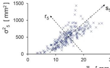
dis-Figure 5.Scatterplot of sample meanz5and sample varianceσ52of calendar month “May” along with the principle componentss5and

r5.

tribution functions, defined as

0−distribution:E[Z] =µ

λ;VAR[Z] = µ

λ2; (14)

Weibull−distribution:E[Z] =λ·0(1+1/ k);

VAR[Z] =λ2·0(1+2/ k)−E[Z]2. (15) The dependence of the two derived parameterszandσ2on each other appears obvious in the case of monthly precip-itation: a high mean is likely to be associated with a high variance and vice versa. Their dependence is exemplary il-lustrated for the calender month “May” in Fig. 5.

The principal component analysis allows for the transfor-mation into the new Cartesian coordinate system with the new coordinates rc(xi)andsc(xi). They are now indepen-dent and subject to a separate interpolation by EDK. A total of 24 (=12×2) interpolations by EDK to the unknown lo-cationxis performed for each selected type of distribution.

3 Results and discussion

The proposed interpolation method of QK, using either a0

distribution (QK-0) or a Weibull distribution (QK-Wei), is implemented and compared to the traditional geostatistical interpolation methods of OK and EDK. The respective per-formances are evaluated by cross-validation for the result-ing estimatorsZ∗and the associated kriging variancesσ_K2. In here, cross-validation eliminates all values z(xi, t )in turns from the input data, and subsequently calculates the estima-torZ∗(xi)and the associated kriging varianceσ_K2(xi)from the remaining data. Only the 32 226 data points of the actu-ally recorded values were considered for the cross-validation and the resulting outcomes are compared to the actual obser-vations.

3.1 Implementation of quantile kriging

The outcomes from the interpolation by OK, EDK and QK-0

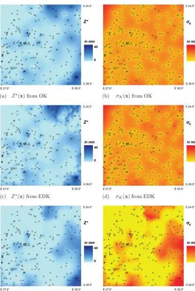
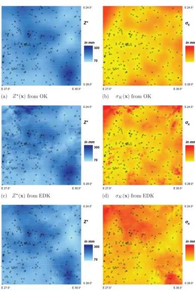
are exemplary displayed and examined for a month with low precipitation and a high dry ratio (August 1993) and a month with high precipitation and a low dry ratio (January 1996). The respective spatial patterns of the estimatorZ∗(x)and the associated standard deviationσK(x)are illustrated in Figs. 6 and 7.

The estimator Z∗ displays similar spatial patterns and value ranges for all the interpolation methods. However, the local contours of the isohyets are more rugged for QK-0

(Figs. 6e and 7e) than for OK (Figs. 6a and 7a), but smoother than for EDK (Figs. 6c and 7c).

QK utilizes elevation for the interpolation of the two dis-tribution parametersϑ1,c andϑ2,c. The two parameters in-corporate information from all time stepstc of the specific calendar monthcand, thus, transfer information over time. They are further combined with the ordinary kriged quan-tilesW (x, t ), leading to more smooth contours of the iso-hyets than EDK (compare Fig. 3). We regard the resulting spatial patterns of QK as more plausible, assuming that the accumulated monthly precipitation is hardly affected by local features in elevation.

The standard deviations σK of the associated estimation error show notable deviations in spatial pattern for the im-plemented interpolation methods. The range of error is no-tably higher for QK (Figs. 6f and 7f) and its spatial pat-terns deviates from the typical, bull-eye-shaped patpat-terns of OK (Figs. 6b and 7b) or EDK (Figs. 6d and 7d).

The estimation error from OK and EDK depends on the spatial configuration of the observation locations xi, their global variance and the selected variogram model. This typ-ical spatial pattern of the error distribution from the ordi-nary kriged quantilesW (x)is converted within QK by the monotonic cdf (Eq. 12). The resultingσK(x)of the original variableZ(x)is, therefore, increased by relatively flat slopes of the cdfs, which are encountered for relatively high val-ues ofW (x). A relationship between the magnitude of the estimatorZ∗ and the magnitude of the associated standard deviationσKis suggested by Figs. 6 and 7.

3.1.1 Relationship between estimator and standard deviation

A relationship between the magnitude of the estimatorZ∗

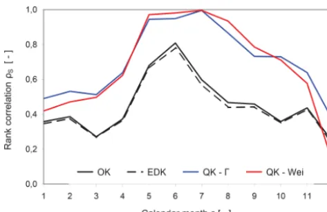
Figure 8.Evolution of the Spearman rank correlation coefficientρS between the estimatorZ∗and the standard deviationσK.

defined as

ρS= (16)

n P

i=1

(rg(Z∗(x_i, t ))−rg_Z∗)×(rg(σ_K(x_i, t ))−rg_σ) s

n P

i=1

(rg(Z∗_(x

i, t ))−rgZ∗)2× n P

i=1

(rg(σK(xi, t ))−rgσ)2 ,

where rg(Z∗(x_i, t ))and rg(σK(xi, t ))are the ranks of the es-timatorZ∗ and the associated standard deviationσK within a set of data, while rg_Z∗ and rg_σ are the respective average ranks. The non-parametric Spearman rank correlationρS de-scribes the monotonic relation between the estimatorZ∗and estimation standard deviation σK, ranging from −1 (nega-tive) to +1 (positive) with 0 indicating its absence. A set of data consists of all nvalues of the corresponding calen-dar monthc. The evolution of the Spearman rank correla-tion coefficientρS over all 12 calendar months is displayed in Fig. 8.

The rank correlation varies over the calendar months for all implemented interpolation methods and reach their sea-sonal maximums in June or July (Fig. 8), being characterized by a high dry ratio and low precipitation.

An improvement in the relationship between the estimator

Z∗and the associated standard deviationσKcan be observed for QK-0and QK-Wei, exhibiting superior rank correlation coefficients for all calender months with the exception of QK-Wei in December (Fig. 8). QK-0deploys the strongest relation during the wetter months from October to March, while QK-Wei is superior from May to September. The re-sulting spread of the error distribution is increased by de-creasing slopes of the theoretical cdfs (Eqs. 12 and 13) and vice versa. The slope is effectively the probability density function (pdf). Both selected theoretical distributions imply a monotonic decrease in their respective pdfs for small pa-rameters, being typically encountered during the dry season, and evoke a higher spread of the error distribution for higher

they influence the linear estimatorZ∗and the standard devi-ationσK by the same extent. Therefore, the non-parametric Spearman descriptor hardly differentiates between OK and EDK.

3.2 Cross-validation of the estimator

The estimatorZ∗(xi, tj) from the cross-validation is eval-uated by six objective functions: the Pearson correlation coefficientρ, the Nash–Sutcliffe efficiency coefficient NSE (Nash and Sutcliffe, 1970), the overall bias B1 and the root mean square error (RMSE) are complemented by the tempo-ral bias B2 and the spatial bias B3 (Bárdossy and Pegram, 2012), which are defined as

ρ= ni

P

i=1 J

P

j=1

(Z∗(xi, tj)−Z

∗

)×(z(xi, tj)−z)

s

ni

P

i=1 J

P

j=1

h Z∗_(x

i, tj)−Z

∗i2

× ni

P

i=1 J

P

j=1

z(xi, tj)−z

2

[−] (17)

NSE=1− ni X i=1 J X j=1

z(xi, tj)−Z∗(xi, tj) 2

z(xi, tj)−z

2 [−] (18)

B1= 1 ntot ni X i=1 J X j=1

z(xi, tj)−Z∗(xi, tj)[mm] (19)

B2= 1 ntot ni X i=1 " _J X j=1

z(xi, tj)−Z∗(xi, tj) #2

h

mm2i (20)

B3= 1 ntot J X j=1 " _n i X i=1

z(xi, tj)−Z∗(xi, tj) #2

h

mm2i (21)

RMSE= v u u t 1 ntot ni X i=1 J X j=1

z(xi, tj)−Z∗(xi, tj) 2

[mm] (22)

whereJ is the number of time steps, ni is the number of observation locations andntot is the total number of cross-validated observations. Note that the cross-validation for only one time step (J=1) would yield the following rela-tions:ntot×B12=B3 and B2=RMSE2.

3.2.1 Summary results

dry season (calender months: 4–9) and wet season (calender months: 1–3 and 10–12) are given in Table 1.

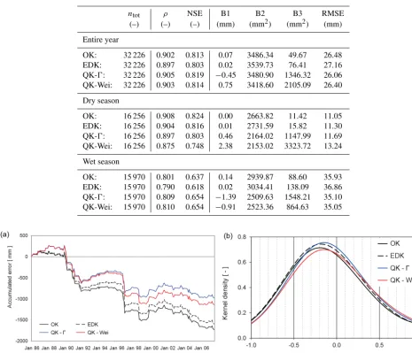
The total values of the correlation coefficientρ, the NSE coefficient, the temporal bias B2 and the RMSE are better for QK-0and QK-Wei than for OK and EDK, evoking from a superior performance especially during the wet season when not many of many zero values are present (see Table 1).

Complementary, OK and EDK have superior values for the biases B1 and B3 as a result of the implicit definition as best linear and unbiased estimator. OK (and to some extent EDK) optimize the spatial bias B3 for a given month by adapting their global mean to the observed mean, according to Eq. (1) (Eq. 3). However, this evokes a systematic underestimation in regions of high precipitation and a systematic overestima-tion in regions of low precipitaoverestima-tion. Therefore, a temporal bias B2 accumulates for a location, which consistently ex-periences extreme precipitation over time. Especially during the wet season, QK outperforms OK and EDK with respect to the temporal bias. The following investigations on raingauge “Wilgervier” exemplary serve as illustration for the evolution of a temporal bias.

3.2.2 Temporal bias at raingauge “Wilgervier”

Raingauge “Wilgervier” (i=125, see Fig. 3) records a rela-tively high monthly precipitation of 70.1 mm in average com-pared to the average monthly precipitation of 54.7 mm in the entire domain.

The evolution of the temporal bias B2 at raingauge “Wilgervier” is calculated from cross-validation according to Eq. 20 and illustrated in Fig. 9 (left). In addition, the rel-ative estimation error r is estimated from the 218 (out of the 264 possible) original observations at “Wilgervier”, be-ing defined as

r(x125, tj)=

Z∗(x125, tj)−z(x125, tj) z(x125, tj)

. (23)

The 218 values ofr(x125)are smoothed by a Gaussian ker-nel with a defined range dG (=0.35). The distribution of the relative estimation errors should ideally be symmetrical around zero. However, the respective distributions are trun-cated due the confinement to r≥ −1 for the variable of monthly precipitation. The smoothed distributions are fac-tually a summary of the estimation errors and are illustrated in Fig. 9 (right).

OK displays the highest systematic underestimation over time (Fig. 9 left) and the relative estimation errors have a mode of −20 % (Fig. 9 right). EDK slightly improves the systematic bias of the interpolation, but the relative error distribution still possess a mode of −15 %. QK-0and QK-Wei can further improve the systematic underestimation over time and exhibit error distributions with modes of−12 %, and−10 % respectively.

Raingauge “Wilgervier” illustrates that OK and EDK might optimize the spatial bias (Table 1), but they are

ham-pered to minimize the temporal bias in locations of extreme observations. QK, as a spatio-temporal interpolation method, is capable of reducing the temporal bias within regions of rel-atively high (or low) precipitation, which is potentially im-portant for possible successive water balance considerations. 3.2.3 Cross-validation for different calendar months

The effects of the increased occurrence of zero-value obser-vations on the Pearson correlation coefficientρ(Eq. 17) and the RMSE (Eq. 22) is exemplary examined next. The respec-tive values are calculated for each calender month from the cross-validation and are illustrated in Fig. 10 along with the dry ratio (Fig. 4).

QK-0 and QK-Wei display improved values in compar-ison to OK and EDK for the two selected objective func-tions from October to March (Fig. 10). However, their per-formance deteriorates from May to September, when many zero-value observations are present, indicated by a dry ra-tio of at least 25 % or above. The correlara-tion coefficientρ

plunges in July for both versions of QK (Fig. 10 left) and the respective RMSE shows a similar qualitative behavior (Fig. 10 right).

The performance of QK is considerably influenced by the dry ratio. The presence of many zero values in the data leads to very steep or nearly vertical theoretical cdfs, hampering the allocation of the quantiles to the respective precipitation values.

3.3 Cross-validation of the uncertainty

The estimated error distribution of the estimatorZ∗(x)is de-scribed by the associated standard deviationσK(x)as a mea-sure of associated uncertainty. The quality of the uncertainty from the cross-validation is assessed by two objective func-tions: the adapted linear error in the probability space LEPS (Ward and Folland, 1991) and a test on uniformity (Bárdossy and Li, 2008).

LEPS compares the values of the estimatorZ∗(xi, t )and the observationz(xi, t )within the estimated cdfFZ∗ of the error distribution as

LEPS= 1 ntot · ntot X i=1

FZ∗(z(x_i, t ))−FZ∗(Z∗(x_i, t )), (24)

LEPS is defined on the interval[0,1]: low values indicate a higher probability for the observation to originate from the estimated probability density distribution and vice versa. The average over the differences of all observationsntotyields the overall LEPS value.

The test on uniformity verifies the estimated, conditional distribution FZ∗ by calculating its value F_Z∗(z(x_i, t )) for every original observationz(xi, t ). The resulting values (or quantiles) should be uniformly distributed on the interval

QK-Wei: 32 226 0.903 0.814 0.75 3418.60 2105.09 26.40

Dry season

OK: 16 256 0.908 0.824 0.00 2663.82 11.42 11.05

EDK: 16 256 0.904 0.816 0.01 2731.59 15.82 11.30

QK-0: 16 256 0.897 0.803 0.46 2164.02 1147.99 11.69

QK-Wei: 16 256 0.875 0.748 2.38 2153.02 3323.72 13.24

Wet season

OK: 15 970 0.801 0.637 0.14 2939.87 88.60 35.93

EDK: 15 970 0.790 0.618 0.02 3034.41 138.09 36.86

QK-0: 15 970 0.809 0.654 −1.39 2509.63 1548.21 35.10 QK-Wei: 15 970 0.810 0.654 −0.91 2523.36 864.63 35.05

Figure 9.Errors of the estimatorZ∗(x₁₂₅)at raingauge “Wilgervier”: evolution of temporal bias B2 over the study period(a)and smoothed distribution of the relative estimation errorr(b).

frequency. The deviation from uniformity is quantified by theχ2- test variable as the sum of the relative squared differ-ences between uniformity and empirical distribution, ranging from zero (perfect) to nine (improper).

3.3.1 Summary results

The values of the two objective functions from cross-validation of all 32 226 original observations of the entire year, and divided into dry (calender months: 4–9) and wet season (calender months: 1–3 and 10–12) are displayed in Table 2.

The best overall LEPS values are received from the tradi-tional EDK and OK (Table 2). QK-Wei is superior to QK-0, but both versions of QK are displaying higher LEPS values

than OK or EDK, originating from the dry season when many zero values are present in the data.

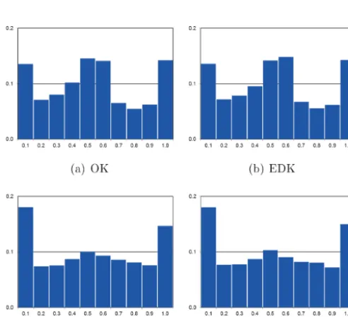
However, theχ2-test variables (Table 2) exhibit a reverse hierarchy among the implemented interpolation methods: QK is superior during the dry season and similar during the wet season. Theχ2-test variables should be read in conjunc-tion with the corresponding histograms of the FZ∗ values (Fig. 11). Note that the outer classes of the histograms host all the observationsz(xi, t ), which are situated outside the estimated distribution. These classes exhibit the largest devi-ation from the ideal uniform distribution.

Table 2.Summary results from the cross-validation of the estimation error for the entire year, and split into dry (calender months: 4–9) and wet (calender months: 1–3 and 10–12) season.

ntot LEPS χ2 ntot LEPS χ2 ntot LEPS χ2

(–) (–) (–) (–) (–) (–) (–) (–) (–)

Entire year Dry season Wet season

OK: 32 226 0.25 0.13 16 256 0.19 0.32 15 970 0.30 0.17

EDK: 32 226 0.24 0.13 16 256 0.19 0.33 15 970 0.30 0.17

QK-0: 32 226 0.32 0.11 16 256 0.36 0.10 15 970 0.28 0.18

QK-Wei: 32 226 0.26 0.12 16 256 0.27 0.10 15 970 0.25 0.18

Figure 10.Evolution of two objective functions for the estimator over the 12 calendar months: Correlation coefficientρ(a)and RMSE(b). Note that the dry ratio (dashed brown line) is indicated as a percentage on the right axis.

Figure 11.Histograms for theFZ∗-values of four different interpo-lation methods.

(Table 2 and Fig. 11) due to their implicit affinity in defini-tion.

3.3.2 Cross-validation for different calendar months

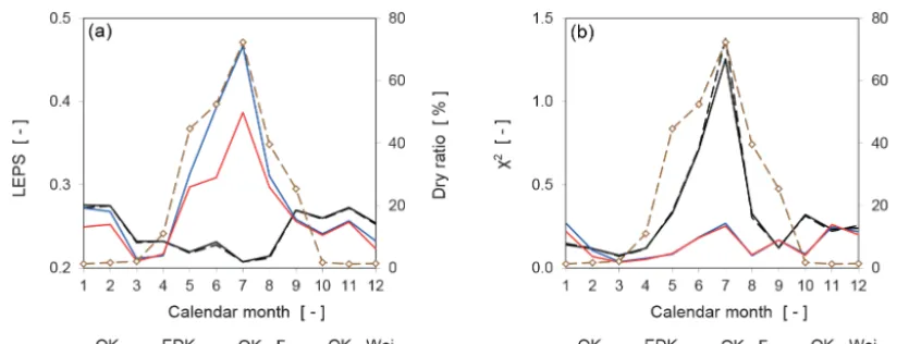
The effect of many zero-value observations on the error dis-tribution is investigated by the differentiation into calendar months. The objective functions are recalculated accordingly and illustrated in Fig. 12.

The temporal evolution of the LEPS values for the two ver-sions of QK is influenced by the presence of many zero-value observations. QK-0and QK-Wei exhibit LEPS values supe-rior to OK and EDK from September to April, characterized by a dry ratio of less than 26 % (Fig. 12, left). However, the performance of QK deteriorates from May to August when many zero-value observations are present. This dependence explains the overall inferior LEPS values for QK in Table 2. The LEPS values for OK and EDK are hardly influenced by the dry ratio (Fig. 12 left) and show a congruent behavior.

Figure 12.Evolution of the two objective functions for the error distribution over 12 calendar months: LEPS(a)andχ2(b). Note that the dry ratio (dashed brown line) is indicated as a percentage on the right axis.

The cross-validation for the uncertainty suggests an im-provement by QK under the prerequisite of a low dry ratio within the input data. This improvement is attributed to the wider range of the error distribution and the increased rela-tion between the magnitude of the estimator and the spread of the distribution (see Sect. 3.1).

4 Conclusions

The geostatistical interpolation method of QK addresses the spatial non-stationarity of a variable of interest by its con-version into quantiles and defining distribution parameters. The spatial–temporal description of the variable by QK is a novelty in applied geostatistics and can be regarded as a temporal extension of probability kriging. Therefore, the pro-posed method could be extended to spatially aggregated vari-ables of streamflows, requiring, however, further investiga-tions. The proposed method accommodates skewed marginal distributions and converts them into an ideal Gaussian distri-bution prior to interpolation as a major theoretical advantage over the traditional OK or EDK. QK describes an asymmetri-cal distribution of the random variableZ(x)by the nonlinear estimatorZ∗(x)and the estimation varianceσ_K2(x)of the er-ror. QK further establishes a relation between the magnitude of both descriptors.

The variable of monthly precipitation, observed at 226 raingauges over 264 consecutive time steps, serves as in-put data. We selected the two-parametric0distribution and Weibull distribution, because they are defined on the interval

[0,∞]and are suitable to describe the variable of monthly precipitation. The selected distributions are fitted to the ob-servations of a specific calendar month, implying an absence of temporal dependence between two sample members (e.g., between the monthly precipitation of December 2002 and December 2003). However, QK does accommodate tempo-ral independence between consecutive observations, unlike existing spatio-temporal kriging methods. In general, other

types of distributions, with a higher number of parameters could be selected, especially in case of other variables of in-terest. Finally, we used elevation as external drift, both for the interpolation of the parameters within QK as well as for the reference EDK.

The cross-validation of the estimator revealed an improve-ment for most of the selected objective functions. In partic-ular, QK addresses the temporal bias, which remains unat-tended by the traditional geostatistical methods, which only optimize the mean spatial bias. In case of the estimator,

QK-0performs slightly better than QK-Wei for most of the se-lected objective functions. The cross-validation of the asso-ciated uncertainty shows an improvement by QK in the de-scription of the distribution of the estimation errors in com-parison to the traditional geostatistical interpolation methods. However, its performance depends on the percentage of zero values in the input data and declines when many zero values are present. In general, QK-Wei shows a superior estimation of the associated uncertainty than QK-0.

Code availability. Respective codes can be obtained from the cor-responding author.

Data availability. Precipitation and elevation data can be obtained from the respective sources mentioned in Sect. 2.3.1

Author contributions. HL and AB set up, collaborated and de-signed the study. HL performed the computational work and wrote the paper. AB and HL interpreted the results and replied to the com-ments from the reviewers.

Acknowledgements. This research was executed at the Institute for Modeling Hydraulic and Environmental Systems of the University of Stuttgart.

Review statement. This paper was edited by Sally Thompson and reviewed by Marc F. Muller and two anonymous referees.

References

Adhikary, P. P., Dash, C. J., Bej, R., and Chandrasekharan, H.: Indicator and probability kriging methods for delineating Cu, Fe, and Mn contamination in groundwater of Najafgarh Block, Delhi, India, Environ. Monit. Assess., 176, 663–676, https://doi.org/10.1007/s10661-010-1611-4, 2011.

Ahmed, S. and deMarsily, G.: Comparison of geostatistical meth-ods for estimating transmissivity using data on transmissivity and specific capacity, Water Resour. Res., 23, 1717–1737, 1987. Armstrong, M.: Basic Linear Geostatistics, Springer, available

at: http://books.google.de/books?id=-9vp1lVuMCsC, Springer Berlin Heidelberg, 1998.

Basistha, A., Arya, D. S., and Goel, N. K.: Spatial Distribu-tion of Rainfall in Indian Himalayas – A Case Study of Uttarakhand Region, Water Resour. Manag., 22, 1325–1346, https://doi.org/10.1007/s11269-007-9228-2, 2008.

Bourennane, H., King, D., and Couturier, A.: Comparison of krig-ing with external drift and simple linear regression for predictkrig-ing soil horizon thickness with different sample densities, Geoderma, 97, 255–271, https://doi.org/10.1016/S0016-7061(00)00042-2, 2000.

Bárdossy, A. and Li, J.: Geostatistical interpolation using copulas, Water Resour. Res., 44, 1–15, 2008.

Bárdossy, A. and Pegram, G.: Interpolation of precipitation un-der topographic influence at different time scales, Water Resour. Res., 49, 4545–4565, https://doi.org/10.1002/wrcr.20307, 2012. Carr, J. R. and Mao, N.-H.: A general form of probability kriging for

estimation of the indicator and uniform transforms, Math. Geol., 25, 425–438, https://doi.org/10.1007/BF00894777, 1993. Chilès, J.-P. and Delfiner, P.: Geostatistics: modeling spatial

uncer-tainty, Wiley, New York, 1999.

Cole, S. J. and Moore, R. J.: Hydrological

mod-elling using raingauge- and radar-based estima-tors of areal rainfall, J. Hydrol., 358, 159–181, https://doi.org/10.1016/j.jhydrol.2008.05.025, 2008.

DWA: Hydrological Information System (HIS), available at: http: //www.dwa.gov.za/Hydrology/ (last access: 5 October 2008), 2008.

Gabellani, S., Boni, G., Ferraris, L., von Hardenberg, J., and Provenzale, A.: Propagation of uncertainty from rainfall to runoff: A case study with a stochastic rain-fall generator, Adv. Water Resour., 30, 2061–2071, https://doi.org/10.1016/j.advwatres.2006.11.015, 2007.

Goovaerts, P.: Geostatistical approaches for incorporating elevation into the spatial interpolation of rainfall, J. Hydrol., 228, 113–129, https://doi.org/10.1016/S0022-1694(00)00144-X, 2000. Goovaerts, P., AvRuskin, G., Meliker, J., Slotnick, M., Jacquez, G.,

and Nriagu, J.: Geostatistical modeling of the spatial variabil-ity of arsenic in groundwater of southeast Michigan, Water

Re-sour. Res., 41, w07013, https://doi.org/10.1029/2004WR003705, 2005.

Journal, A. and Alabert, F.: Non-Gaussian data expan-sion in the Earth Sciences, Terra Nova, 1, 123–134, https://doi.org/10.1111/j.1365-3121.1989.tb00344.x, 1989. Journel, A. G.: Nonparametric estimation of spatial distributions,

Journal of the International Association for Mathematical Geol-ogy, 15, 445–468, https://doi.org/10.1007/BF01031292, 1983. Kobold, M. and Sušelj, K.: Precipitation forecasts and their

uncer-tainty as input into hydrological models, Hydrol. Earth Syst. Sci., 9, 322–332, https://doi.org/10.5194/hess-9-322-2005, 2005. Lebrenz, H. and Bárdossy, A.: Estimation of the

Var-iogram Using Kendall’s Tau for a Robust Geosta-tistical Interpolation, J. Hydrol. Eng., 22, 04017038, https://doi.org/10.1061/(ASCE)HE.1943-5584.0001568, 2017. Lee, J.-J., Jang, C.-S., Wang, S.-W., and Liu, C.-W.: Evaluation of

potential health risk of arsenic-affected groundwater using indi-cator kriging and dose response model, Sci. Total Environ., 384, 151–162, https://doi.org/10.1016/j.scitotenv.2007.06.021, 2007. Lynch, S.: Development of a Raster Database of Annual, Monthly

and Daily Rainfall for Southern Africa, Report 1156/1/03, Water Research Commission, Pretoria, RSA, 2004.

Matheron, G.: Traité de Géostatistique Appliquée, Mémoires du Bureau de Recherches Géologiques et Minières, vol. I, p. 333, Paris, 1962.

Matheron, G.: Les variables régionalisées et leur estimation: une application de la théorie des fonctions aléatoires aux sciences de la nature, PhD thesis, Université de Paris, Paris, 1965.

Mitchell, T. D. and Jones, P. D.: An improved method of con-structing a database of monthly climate observations and as-sociated high-resolution grids, Int. J. Climatol., 25, 693–712, https://doi.org/10.1002/joc.1181, 2005.

Mosthaf, T. and Bárdossy, A.: Regionalizing nonparametric models of precipitation amounts on different temporal scales, Hydrol. Earth Syst. Sci., 21, 2463–2481, https://doi.org/10.5194/hess-21-2463-2017, 2017.

Motaghian, H. and Mohammadi, J.: Spatial Estimation of Satu-rated Hydraulic Conductivity from Terrain Attributes Using Re-gression, Kriging, and Artificial Neural Networks, Pedosphere, 21, 170–177, https://doi.org/10.1016/S1002-0160(11)60115-X, 2011.

Moulin, L., Gaume, E., and Obled, C.: Uncertainties on mean areal precipitation: assessment and impact on stream-flow simulations, Hydrol. Earth Syst. Sci., 13, 99–114, https://doi.org/10.5194/hess-13-99-2009, 2009.

Nash, J. and Sutcliffe, J.: River flow forecasting through conceptual models part I – A discussion of principles, J. Hydrol., 10, 282– 290, https://doi.org/10.1016/0022-1694(70)90255-6, 1970. Rosenblueth, E.: Point estimates for probability moments, P. Natl.

Acad. Sci. USA, 72, 3812–3814, 1975.

Snepvangers, J., Heuvelink, G., and Huisman, J.: Soil water con-tent interpolation using spatio-temporal kriging with external drift, Geoderma, 112, 253–271, https://doi.org/10.1016/S0016-7061(02)00310-5, 2003.