www.hydrol-earth-syst-sci.net/15/3411/2011/ doi:10.5194/hess-15-3411-2011
© Author(s) 2011. CC Attribution 3.0 License.
Earth System
Sciences
Catchment classification: hydrological analysis of catchment
behavior through process-based modeling along a climate gradient
G. Carrillo1, P. A. Troch1, M. Sivapalan2, T. Wagener3, C. Harman2, and K. Sawicz3
1University of Arizona, Tucson, AZ,, USA
2University of Illinois at Urbana-Champaign, Urbana, IL, USA 3Pennsylvania State University, University Park, PA, USA
Received: 30 March 2011 – Published in Hydrol. Earth Syst. Sci. Discuss.: 9 May 2011 Revised: 30 July 2011 – Accepted: 28 September 2011 – Published: 16 November 2011
Abstract. Catchment classification is an efficient method to
synthesize our understanding of how climate variability and catchment characteristics interact to define hydrological re-sponse. One way to accomplish catchment classification is to empirically relate climate and catchment characteristics to hydrologic behavior and to quantify the skill of predicting hydrologic response based on the combination of climate and catchment characteristics. Here we present results using an alternative approach that uses our current level of hydrolog-ical understanding, expressed in the form of a process-based model, to interrogate how climate and catchment character-istics interact to produce observed hydrologic response. The model uses topographic, geomorphologic, soil and vegeta-tion informavegeta-tion at the catchment scale and condivegeta-tions pa-rameter values using readily available data on precipitation, temperature and streamflow. It is applicable to a wide range of catchments in different climate settings. We have devel-oped a step-by-step procedure to analyze the observed hy-drologic response and to assign parameter values related to specific components of the model. We applied this proce-dure to 12 catchments across a climate gradient east of the Rocky Mountains, USA. We show that the model is capable of reproducing the observed hydrologic behavior measured through hydrologic signatures chosen at different temporal scales. Next, we analyze the dominant time scales of catch-ment response and their dimensionless ratios with respect to climate and observable landscape features in an attempt to explain hydrologic partitioning. We find that only a limited
Correspondence to: G. Carrillo ([email protected])
number of model parameters can be related to observable landscape features. However, several climate-model time scales, and the associated dimensionless numbers, show scal-ing relationships with respect to the investigated hydrologi-cal signatures (runoff coefficient, baseflow index, and slope of the flow duration curve). Moreover, some dimensionless numbers vary systematically across the climate gradient, pos-sibly as a result of systematic co-variation of climate, vege-tation and soil related time scales. If such co-variation can be shown to be robust across many catchments along differ-ent climate gradidiffer-ents, it opens perspective for model param-eterization in ungauged catchments as well as prediction of hydrologic response in a rapidly changing environment.
1 Introduction
3412 G. Carrillo et al.: Hydrological analysis of catchment behavior through process-based modeling a region. However, catchment classification is only complete
if we understand why certain catchments belong to certain groups of hydrologic behavior, such that we have the means to classify ungauged catchments into their most likely group of behavior.
One way to accomplish catchment classification is to em-pirically relate climate and catchment characteristics to hy-drologic behavior and to quantify the uncertainty of pre-dicting the hydrologic response based on a combination of climate and catchment characteristics. Such a classifica-tion system and the related predicclassifica-tion uncertainty will be conditioned by the selection of hydrologic signatures and climate/catchment characteristics, and may result in differ-ent classifications depending on the objective of classifica-tion (e.g. water balance particlassifica-tioning, ecological services). In any case, we can call this approach the top-down approach since it is based on measurable hydrologic drivers/responses and landscape features. The measure of uncertainty quanti-fies the probability of misclassification, and provides insight about how much information is contained in the selected cli-mate and catchment characteristics concerning hydrologic response (Snelder et al., 2005; Oudin et al., 2010). Since there are important surface and subsurface properties that cannot be readily measured or translated into hydrologically relevant information, the uncertainty of classification reflects in part (the lack of) the amount of cross-correlation between observable landscape properties (e.g. vegetation type) and unobservable landscape characteristics (e.g. rooting depth).
An alternative approach, that can partially alleviate the above-mentioned issue of observability, uses our current level of hydrological understanding, expressed in the form of a process-based model, to interrogate how climate and catchment characteristics interact to produce the observed hydrologic response (Sivakummar, 2008). Assuming an ap-propriate process-based model can be constructed for a wide range of catchments, we can use it to analyze the relation-ships between hydrologic response and catchment function-ing (Samuel et al., 2008). A catchment can be considered as a filter that transforms the climate signal into a hydro-logic response by partitioning, storing and releasing incom-ing energy and water (Black, 1997; Wagener et al., 2007). The different catchment stores (e.g. interception store, root zone store, aquifer store) interact with the different climate fluxes (e.g. rainfall intensity, maximum evapotranspiration) to produce specific time constants of hydrologic behavior (e.g. time to empty root zone store through evapotranspira-tion). The process-based model can thus be a very useful instrument to analyze different portions of the hydrologic response to identify the important time constants of ment functioning. For instance, the recession part of a catch-ment’s hydrograph during the dormant season can be used to inform us about the time constant of aquifer release by matching modeled recession flows using lumped aquifer de-scriptors, such as horizontal hydraulic conductivity or depth to bedrock (Brutsaert and Nieber, 1977; Kirchner, 2009).
Through process-based modeling we can thus obtain esti-mates of hidden catchment characteristics that are not avail-able in the top-down approach, and ask questions about how these catchment characteristics relate to climate gradients.
Once a sufficient set of catchments across the climate-landscape gradients of a specific region have been analyzed using this bottom-up approach, we can use the model pa-rameters to explain observed hydrologic similarity. Certain model parameters can be prescribed based on observable landscape characteristics (e.g. mean catchment slope, dom-inant vegetation type). Others cannot be determined a pri-ori and need to be selected during the hydrologic analysis phase. Such hydrologic analysis should not be considered as an automated calibration procedure but rather as a step-by-step methodology to distill relevant information about differ-ent catchmdiffer-ent functions using appropriate forcing and output variables (Boyle et al., 2000; Yilmaz et al., 2008). The ad-vantage of automated parameter calibration is that it is ob-jective and does not require interaction of the hydrologist with the optimization algorithm (Hogue et al., 2006). The disadvantage is that typical objective functions used to opti-mize model performance cannot guarantee that inappropriate combinations of parameter values lead to sets of “behavioral” models (Fenicia et al., 2007), and the functional role of spe-cific parameters is often not preserved (Wagener et al., 2003). It is the purpose of this paper to present a general method of hydrologic analysis by means of a process-based model to develop a bottom-up catchment classification system that is compatible with and complementary to top-down classifica-tion methods developed elsewhere (Sawicz et al., 2011). In Sect. 2 we present the process-based model to analyze hy-drologic response across many catchment in the USA. The model is built around the hillslope-storage Boussinesq (hsB) equation developed by Troch et al. (2003). It uses geomor-phologic functions to describe hillslope and channel network topology required to compute subsurface and surface rout-ing. We have chosen this modeling approach because (1) it is parsimonious and thus reduces the problem of equifinal-ity (Beven and Freer, 2001), and (2) it was shown that the hsB equation accurately represents saturated subsurface flow and storage dynamics across complex landscapes (Paniconi et al., 2003). In Sect. 3 we describe a step-by-step proce-dure to analyze the observed hydrologic response and to as-sign parameter values related to specific components of the model. It uses different parts of the catchment hydrograph to separate processes in an attempt to reduce parameter un-certainty and to increase the probability to assign a reason-able range of parameter values to different components of the model. In Sect. 4 we apply our hydrologic analysis procedure to 12 catchments selected from the MOPEX (Model Param-eter Experiment) database across a climate gradient in the USA, and present a comparison of hydrologic functioning as revealed by our process-based model. In Sects. 5 and 6 we discuss our results and some shortcomings of the bottom-up approach to catchment classification.
2 Process-based model for hydrologic analysis
2.1 Modeling principles
The model we developed for the purpose of this study is based on the following principles: (1) the model should be process-based such that we can use it to analyze catch-ment behavior derived from routine hydro-meteorological observations at the catchment scale, such as daily dis-charge, temperature and precipitation; (2) the model should be as parsimonious as possible to avoid problems of over-parameterization and equifinality (Beven and Freer, 2001; Wagener and Gupta, 2005) and reduce computer process-ing time; and (3) the model should be applicable to a wide range of catchments across climate and physiographic gra-dients. In order to represent the dominant functions of a catchment we consider hillslopes and channel network as fundamental hydrologic units (Troch et al., 2003). Hillslope land surfaces interact with the atmosphere and partition wa-ter and energy fluxes, and drain surface runoff and subsurface flow into the catchment channel network for routing towards the outlet (i.e. point where discharge is measured). Instead of representing individual hillslopes and how they are con-nected to the channel network, we adopt the modeling ap-proach of Troch et al. (1994) and use the hillslope width function and the channel width function at the catchment scale to represent the geomorphologic structure of the catch-ment. Each catchment is thus characterized by a hillslope width function (probability density function of water enter-ing the catchment at a given flow distance from the channel network; see also Bogaart and Troch, 2006) and a channel width function (probability density function of surface and subsurface flow entering the channel network at a given flow distance from the outlet) that are derived from available dig-ital elevation models (DEMs). Important additional terrain properties such as average hillslope/channel slope are also estimated from available DEMs. Other landscape properties, such as land use-land cover and soils, available from various spatial databases are further used to assign initial values to process parameters that control the different catchment func-tions, such as infiltration and interception.
2.2 Model structure and processes
2.2.1 Hillslope and channel routing
The semi-distributed hillslope-storage Boussinesq (hsB) model, developed by Troch et al. (2003), is used to model perched groundwater dynamics at the hillslope spatial scale: f ∂S
∂t =
khcosα f
∂ ∂x
S Wh
∂S ∂x −
S Wh
∂Wh ∂x
+khsinα ∂S
∂x +f N Wh (1)
whereS (=f Wh(x)h) [m2] is saturated storage at flow dis-tancexfrom the hillslope outlet and at timet,Wh(x)[m] is the hillslope width function at flow distancex [m],h(x, t ) [m] is water depth measured perpendicular to the bedrock, αis bedrock slope angle [◦],kh[m s−s] is the effective lat-eral saturated hydraulic conductivity and f [−] is drain-able porosity. The recharge rate N (x, t ) [m s−1] depends on root zone hydrologic processes at flow distance x and thus varies along the hillslope (see below). It was shown by Paniconi et al. (2003) that this model is an adequate and parsimonious representation of three-dimensional sat-urated subsurface flow along geometrically complex hill-slopes. When saturated storage exceeds the local storage capacity Sc (=f Wh(x)D, where D is maximum perched aquifer depth) the model produces saturation excess overland flow. The partial differential equation is solved numerically for water table dynamics and outflow rate (see Troch et al., 2003 for details).
Some fraction of the total percolation from the root zone (see below) is assigned to enter a fractured bedrock aquifer below the perched groundwater table. We assume the outflow from this bedrock aquifer to sustain drought flow at the out-let, and the aquifer dynamics are represented with a lumped non-linear storage model:
Qb = a Sdb (2)
whereQb[m3s−1] is baseflow from the deep aquifer,Sd[m] is deep aquifer storage anda(units depend on value ofb) and b[−] are aquifer parameters (withb= 1 representing a linear reservoir).
Hillslope runoff (either infiltration excess or saturation ex-cess) draining into the channel network is routed by means of an analytical solution to the linearized de St.-Venant equation of open channel flow:
qc(x, t ) =
x
(2π )1/2dt3/2 exp "
−(x −c t )
2 2 d2t
#
(3) whereqc(x, t ) [s−1] is specific discharge resulting from a Dirac impulse input at flow distancexupstream, and c = (1 +a0) V
d2 = V
3 g S0F2
1 −a02F2
. (4)
The parametersc[m s−1] andd2[m2s−1] are referred to as the absolute celerity or drift velocity and the diffusion coef-ficient, respectively.V [m s−1] is the flow velocity,S0[−] is the channel bed slope,F [−] is the flow’s Froude number,g [m s−2] is the acceleration of gravity anda0[−] is an empiri-cal constant depending on the friction slope parameterization (equals 2/3 if Manning’s equation is used).
The normalized channel width function,Wc(x)[m−1], is defined as:
Wc(x)= 1 LT
3414 G. Carrillo et al.: Hydrological analysis of catchment behavior through process-based modeling whereNc(x)is the number of channel links at a given flow
distance from the catchment outlet andLTis the total channel length. Interpreting the normalized channel width function as the probability density function of receiving lateral inflow at flow distancex from the outlet, the response of the channel network to an instantaneous unit input of water is:
fc(t )= ∞ Z
0
qc(x, t ) Wc(x)dx (6)
withqc(x, t )defined in Eq. (3). This parsimonious model of channel routing can be used to compute discharge at the catchment outlet given lateral inflows through either infiltra-tion or saturainfiltra-tion excess overland flow (assumed to enter the channel network at time of generation). Shallow subsurface flow above a confining soil/bedrock layer draining from the hillslope perched aquifer and deep fractured bedrock base-flow are produced at the catchment outlet and thus do not need to be routed through the channel network (see below).
2.2.2 Root zone water balance
The hillslope perched aquifer interacts with the root zone and exchanges recharge and capillary rise fluxes which depend on root zone moisture content and the depth between the root zone and the local water tableh(x, t ), called the transmission zone. The root zone water balance is given by:
Drz dθrz
dt = i +cr −t −r (7)
whereDrz[m] is depth of the root zone,θrz[−] is volumetric soil moisture content of the root zone,i[m s−1] is infiltration rate at the land surface,cr[m s−1] is capillary rise flux from the perched water table into the root zone,t [m s−1] is tran-spiration from the dry canopy andr[m s−1] is recharge rate from the root zone into the transmission zone. The root zone water balance is solved using a daily time step such that all fluxes are daily averages.
The infiltration rateiis given by:
i = min [pt, ic] (8)
wherept is throughfall rate andicis infiltration capacity of the soil. If throughfall rate exceeds the infiltration capacity surface runoff is produced, which is instantaneously added to the lateral flow into the channel network. The throughfall rate is computed as:
pt = 0 ⇔ω < ωc
pt = p ⇔ ω = ωc (9)
whereω[m] is canopy storage,ωcis canopy storage capacity andpis precipitation rate. The actual canopy storage is com-puted using a simple canopy water balance that accounts for precipitation rate and evaporation from the wet canopy and
is bounded by [0, ωc]. The canopy storage capacity is re-lated to the leaf area index (LAI) of the catchment vegetation according to Dickinson (1984):ωc= 0.0002×LAI.
The infiltration capacity of the soil is modeled by means of the time compression approximation suggested by Milly (1986):
ic = 1 2 kv
1 +
"
−1 +
1 + 1
2 kv 4ic
s2 s
1/2#−1
(10)
wherekv [m s−1] is the vertical hydraulic conductivity, ss [m s−0.5] is the soil sorptivity andIc [m] is the cumulative infiltration since start of rain/snow melt event.
The rate of capillary rise is modeled according to Gard-ner (1958) for steady upward flow from a water table: c = βc
a (Z −9c)b
(11) whereψc[m] is the depth of the capillary fringe,βc[−] is a reduction factor that varies linearly withθrzbetween residual moisture content and saturated moisture content, anda and b are parameters that are related to the Brooks-Corey soil water retention parameters (Eagleson, 1978). Z [m] is the depth (distance) between the bottom of the root zone and the local water table, and thus varies along the hillslope.
Percolation or recharge from the bottom of the root zone is assumed to be solely gravity driven and is computed as:
r = kv θ
rz −θr θs −θr
2+B3B
(12) whereθris residual moisture content andθsis saturated mois-ture content, andBis the Brooks-Corey pore size distribution index.
The transmission zone between root zone and perched aquifer transmits water received from the root zone towards the perched aquifer at a rate defined through Eq. (12) with a transmission zone specific vertical hydraulic conductivity and moisture content. It also transmits capillary rise flux from the perched aquifer to the root zone unaltered, with-out storage of water. The effective depth of the transmission zone is dynamic and depends on the root zone and perched aquifer storage dynamics (Zdecreases asSincreases). The difference between the recharge flux from the transmission zone and the capillary rise flux,cr, defines the net recharge, N, to the shallow aquifer.
2.2.3 Land surface energy balance
Evaporation from wet canopy and transpiration from veg-etation are estimated by means of the land surface energy budget:
Rn = λE +H +G (13)
withRn[W m−2] net radiation,E[kg s−1m−2] vaporization rate,λ[J kg−1] latent heat of vaporization,H [W m−2] sen-sible heat flux andG[W m−2] soil heat flux. Net radiation is estimated from the surface radiation budget accounting for incoming and outgoing shortwave and longwave radiation, depending on surface albedo and emissivity. Since outgo-ing longwave radiation depends on surface temperature, we solve the energy budget iteratively and assume the surface emissivity constant. The latent heat flux can be approximated as (Brutsaert, 2005):
λE = ρcp
λ (ra +rc)
[es(Ts)−ea] (14)
whereρ[kg m−3] is the density of the air,cp[J kg−1K−1] is the specific heat of the air at constant pressure,γ[Pa K−1] is the psychrometric constant,ra[s m−1] is the aerodynamic re-sistance,rc[s m−1] is the canopy (stomatal) resistance,es(Ts) [Pa] is saturated vapor pressure at surface temperatureTs, andea[Pa] is the vapor pressure of the air. The aerodynamic resistance is given by:
ra = 1 u(z) k2
ln
z−d z0
2
(15) withu(z)[m s−1] wind speed at heightz,kis von Karman’s constant (= 0.41), d [m] is zero plane displacement height andz0[m] is the roughness length of the canopy. The sensi-ble heat flux is estimated from:
H = λcp
ra
(Ts −Ta) (16)
whereTa[K] is air temperature.
We solve the land surface energy budget for surface tem-perature at daily time steps such that we can assume the net ground heat flux to be zero. When the canopy is wet (ω >0) the canopy resistance is zero. Evaporation from wet canopy is then given by:
ewc =ωwcE (rc = 0) (17)
andωwc is the areal fraction of wet canopy estimated from Deardorff (1978):
ωwc = (ω/ωc)2/3. (18)
The transpiration rate removing moisture from the root zone is given by (Teuling and Troch, 2005):
t = (1 −ωwc) VRFβt
1 −e−µ·LAIE rs,min
(19) whereVRF [−] is the vegetation root fraction,µ[−] is the vegetation light use efficiency,E(rc,min)[m s−1] is the po-tential vaporization rate using a minimal canopy resistance, βis the transpiration reduction coefficient, given by: βt = max
0,min
1, θrz −θw θc −θw
(20) withθwsoil moisture content at wilting point andθcthe crit-ical moisture content when transpiration reduction starts.
2.2.4 Snow accumulation and melt
We add a simple snow model for catchments with significant snow days (see below). The snow model accumulates all in-coming precipitation in a snow pack when the air temperature is below a certain thresholdTm. When air temperature rises above this threshold temperature, the snow melt rate is given by:
Qm = M (Ta −Tm) (21)
withM[m s−1K−1] a melt coefficient. The daily melt vol-ume is subsequently removed from the stored snow water equivalent in the snow pack and added to the throughfall.
2.3 Model forcing
In this study, we run the model at daily time steps, even though it can be run at shorter time steps (e.g. hourly). Re-quired model forcing are daily precipitation, air temperature, downward short- and longwave radiation, relative humidity, atmospheric pressure and wind speed. Other required model inputs include time evolution of catchment-wide leaf area in-dex (LAI) and albedo. We will discuss the different sources of these input variables in Sect. 4. It should be noted that since we use a semi-distributed version of the hsB-SM model the model forcing data is basin-averaged, and soil and vege-tation type are effectively uniform, as in Woods (2003). This no doubt will add to modeling uncertainty but is unavoid-able in order to keep the number of model parameters to a minimum.
2.4 Characteristic time scales and dimensionless numbers
The different components of the process-based model, in combination with catchment-scale climate forcing, reveal characteristic time scales of hydrologic response that are re-lated to catchment hydrologic functions of partitioning, stor-age, and release of water. Therefore, such characteristic time scales are important indicators of catchment behavior and can help to relate above and below ground landscape charac-teristics to water balance dynamics. They can also be com-bined to form dimensionless numbers that can be related to hydrologic regimes through empirical or analytically derived scaling relations (Berne et al., 2005; Harman and Sivapalan, 2009).
2.4.1 Canopy time scales
The time scale associated with filling up the canopy intercep-tion storage capacity,ωc, is given by:
τcf = ωc
3416 G. Carrillo et al.: Hydrological analysis of catchment behavior through process-based modeling wherepis the average rainfall intensity when it rains. The
time scale associated with emptying the interception storage is given by:
τce = ωc ewc
(23) withewc the average wet canopy evaporation. Obviously, both the average rainfall intensity and average wet canopy evaporation vary throughout the year, such that the seasonal canopy time scales can be either larger or smaller than the annual averages defined above. In any case, the interception storage capacity is at most a few mm such that in most cli-mates the canopy time scales are of the order of a few days at maximum, and typically less than one day. The time scales are also of same order of magnitude and thus their ratio, re-flecting the competition between filling and emptying the in-terception storage, is close to 1.
2.4.2 Snow pack time scales
The characteristic time scale of snowmelt can be defined as: τm =
s Qm
(24) wheres is the average maximum snow accumulation, and Qmis the average snow melt rate during snow melt season. This time scale is important to define what type of runoff gen-eration mechanism is likely to dominate (saturation excess vs. shallow subsurface flow) during snow melt by comparing it with characteristic time scales of root zone and perched aquifer processes (see below).
2.4.3 Root zone time scales
The time scale related to filling the root zone storage by rain-fall is defined as:
τrfr =
Drz θs − θ
pt (25)
whereθis the average soil moisture content of the root zone andptis the average throughfall rate whenTa> Tm. Simi-larly, the time scale related to filling the root zone by snow melt is given by:
τrfs =
Drz θs −θ
Qm +pt (26)
It is possible to specify different average soil moisture con-tents during the rainy season and the snow melt season to re-flect different wetness conditions, if necessary. Time scales related to emptying the root zone storage in the absence of capillary rise are:
τrer =
Drz (θs −θFC) r
τret =
Drz θ −θw
t (27)
whereθFCis soil moisture content at field capacity,r is the average recharge rate andtis the average transpiration rate.
Different combinations of these time scales express com-petition between different processes affecting the water bal-ance dynamics. For instbal-ance, the ratio of the latter two re-veals the competition in the catchment between baseflow generation and vegetation water use.
2.4.4 Transmission zone time scales
As mentioned earlier, the depth of the transmission zone is time variable as it depends on the soil moisture dynamics in the root zone as well as on storage dynamics in the perched aquifer. Nevertheless, an average transmission zone storage capacity can be numerically derived from the model simula-tions and used to define the following time scales of trans-mission zone filling and emptying:
τtf =
Z θs −θ r
τte =
Z (θs − θFC) rt
. (28)
In Eq. (28),Zis average transmission zone depth,θsis satu-rated moisture content of the transmission zone,θis average moisture content andrandrtare average recharge rate from root zone and transmission zone, respectively.
2.4.5 Perched aquifer time scales
Much work has been done on defining characteristic time scales of shallow aquifer dynamics (Brutsaert, 1994; Troch et al., 2004; Berne et al., 2005; Harman and Sivapalan, 2009). The characteristic time scale of advection-driven (kinematic) flow in perched aquifers is given by (Berne et al., 2005; Har-man and Sivapalan, 2009):
τU =
L f
2kh(sinα −acpD cosα)
(29) whereLis hillslope length (maximum flow distance between divide and nearest channel), pD is average saturated thick-ness, and ac is the rate of con/divergence of the hillslope width function. Likewise, the characteristic time scale of diffusion-driven flow is given by:
τK =
L2f 4khpD cosα
(30) Their ratio,τK/τU, defines the hillslope P´eclet number (Pe; Berne et al., 2005) and high values of Pe indicate that shallow subsurface flow is mainly dominated by gravity drainage.
Harman and Sivapalan (2009) extended the similarity framework of Berne et al. (2005) to account for the respon-siveness of the hillslope subsurface flow to temporal variabil-ity of the recharge events, as well as for the effects of lower
boundary condition of hillslope drainage. They used the con-cept of hydrologic regimes of Robinson and Sivapalan (1997) to develop a hillslope subsurface flow classification system based on the Pe number and the dimensionless characteristic time of recharge events:
πr = τr τhc
(31) whereτr is the average storm duration and τhc is the con-centration time of the hillslope. Either the advection or the diffusion time scale defined above can be used to estimate the hillslope concentration time. Their classification system defines slow/fast, advection/diffusion dominated subsurface flow, depending on the numerical value of Pe (below 1: dif-fusion; above 1: advection) andπr(below 1: slow; above 1: fast, although the separation between fast and slow flow in the diffusion dominated case depends on the boundary con-dition assumed: fixed (small) flow depth vs. kinematic).
2.4.6 Fractured bedrock time scales
Time scales for non-linear reservoirs representing baseflow dynamics have been proposed by Woods (2003). In many cases, the master baseflow recession curve of a given catch-ment converges to a straight sloping line in semi-logarithmic plots of ln(Qb)versus time, indicating that most deep aquifer
dynamics are best represented by a linear reservoir equation withb= 1. In that case, the characteristic time scale of deep (fractured bedrock) aquifer dynamics is given by 1/a, the reservoir time constant.
2.4.7 Channel network time scales
The advective characteristic time scale of channel flow is given by:
τc = Lc
V (32)
whereLcis flow length along the channel network from the centroid to the outlet and V is average flow velocity. Ob-viously, the channel flow Froude number is an appropriate dimensionless number to characterize the flow regime.
3 Model identification procedure
3.1 Linking parameter values to dominant process
behavior
The above-described hydrologic model is one of many alter-native process-based models that can be formulated to de-scribe different surface and subsurface stores and their inter-actions that generate streamflow (Jothityangkoon and Siva-palan, 2009; Clark et al., 2008). Within the context of such models, routine hydro-meteorological observations can be analyzed to inform us about the different catchment functions
of partitioning, storage and release of incoming water and en-ergy fluxes. During different parts of the hydrologic response not all components of the model are equally active, such that one can link parameter values to specific storage dynamics to avoid unwanted parameter interactions often encountered in automatic calibration procedures. In the following we de-scribe a step-by-step procedure of linking model parameters to specific hydrologic responses generated by the proposed model. This procedure can easily be modified when other process-based models are used.
3.1.1 Dormant vs. growing season
First, we divide the hydrologic year into two periods: one when the vegetation is dormant and one when the vegeta-tion is active (growing season). This decision is based on analyzing the average leaf area index (LAI) curve derived from several years of remote sensing observations at the catchment scale. In this study we use MODIS (Moderate Resolution Imaging Spectroradiometer; http://modis-land. gsfc.nasa.gov/lai.htm) data and more specifically the LAI product available at https://lpdaac.usgs.gov/lpdaac/products/ modis products table from 2000 to 2008. From the annual signals of LAI the average LAI curve is derived and subse-quently rescaled using the minimum and maximum average LAI. The hydrologic year is then separated into the dormant season and growing season using the time instances when the rescaled LAI curve crosses the 50 % cut-off level (Fig. 1). This method is similar to the phenology model for monitor-ing vegetation responses developed by White et al. (1997), and seems to be able to capture the inflexion points of the average LAI curve well.
3.1.2 Step 1: baseflow recession and aquifer dynamics
An obvious starting point for hydrologic analysis of catch-ment response is when the catchcatch-ment is non-driven and re-laxes from previous hydro-meteorological fluxes that have replenished some/all stores. In order to isolate several possi-ble release fluxes from the catchment it is best to start focus-ing on baseflow recessions durfocus-ing the dormant season. Such recession hydrographs will be minimally affected by root wa-ter uptake and subsequent transpiration losses and thus can be considered mainly controlled by aquifer properties. Our process-based model considers two separate aquifer stores: the near-surface perched aquifer that develops during wet period above a confining layer (i.e. fractured bedrock with reduced vertical hydraulic conductivity), and a deep aquifer that receives a fraction of all percolation water from the root zone (i.e. a fractured bedrock aquifer). To relate baseflow recessions to these aquifer stores we perform a baseflow sep-aration as follows:
Qb(t ) = εQb(t −1)+ 1 −ε
3418 G. Carrillo et al.: Hydrological analysis of catchment behavior through process-based modeling
47
Figure 1
: Illustration of average leaf area index (LAI) curve derived from 9 years of MODIS
observations over Tygart River Valley catchment. A cut-off level of 50% of the rescaled LAI curve
is used to separate the dormant and the growing season.
Fig. 1. Illustration of average leaf area index (LAI) curve derived from 9 years of MODIS observations over Tygart River Valley catchment. A cut-off level of 50 % of the rescaled LAI curve is used to separate the dormant and the growing season.
48
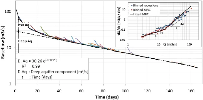
Figure 2: Illustration of derivation of the master recession curve (MRC) for San Marcos, TX catchment and the separation of recession flow derived from the perched and the bedrock aquifer. The inset shows a Brutsaert-Nieber plot of recession rates versus baseflow. The lower end reveals
[image:8.595.130.467.62.209.2]the linear reservoir response of the deep aquifer whereas the upper end shows the non-linear recession characteristics against which the hillslope-storage Boussinesq equation is calibrated.
Fig. 2. Illustration of derivation of the master recession curve (MRC) for San Marcos, TX catchment and the separation of recession flow derived from the perched and the bedrock aquifer. The inset shows a Brutsaert-Nieber plot of recession rates versus baseflow. The lower end reveals the linear reservoir response of the deep aquifer whereas the upper end shows the non-linear recession characteristics against which the hillslope-storage Boussinesq equation is calibrated.
with Q(t ) total streamflow at time t, Qb the computed baseflow contribution to total streamflow (Qb≤Q), andε a low-pass filter parameter (Arnold and Allen, 1999; Eck-hardt, 2005). The filter parameterεis set for all catchments at 0.925. Since the purpose of the study is to address hy-drologic similarity across a climate gradient, the selection of a different cut-off level would not change the relative dif-ferences between the catchments (a desired characteristic of the data manipulation), but obviously will affect to some de-gree the absolute values. Next, all recession periods during the dormant season are selected for recession curve analy-sis (Fig. 2). The catchment master recession curve (MRC) is constructed by time shifting individual recession curves to match the lower end of the baseflow values, and pro-gresses from low to high baseflow values. This procedure is described in more detail in Posavec et al. (2006). Subse-quently, the MRC is defined as the smoothed lower envelope
of all observed recession curves. According to our concep-tual model of baseflow generation, we can consider the early part of the MRC as being composed of both perched and deep aquifer contributions while the late part of the MRC is solely composed of deep aquifer contributions. Therefore, starting from the low flow end of the MRC, the deep aquifer parame-ters are estimated to match that part of the MRC. In all appli-cations of the model to our study sites (see Sect. 4) we have observed that the lower end of the MRC can be approximated by means of a linear reservoir model, characterized by a time constant of storage release given by the reciprocal value of the slope of the linear regression line through the lower end of the MRC (Fig. 2). Parameter values are estimated us-ing the downhill Simplex method (Nelder and Mead, 1965) with least square error objective function. The inset of Fig. 2 shows a Brutsaert-Nieber plot of recession rates versus base-flow of binned observations and MRC. The lower end reveals
[image:8.595.127.467.258.426.2]the linear reservoir response of the deep aquifer whereas the upper end shows the non-linear recession characteristics against which the hillslope-storage Boussinesq equation is calibrated.
Using the deep aquifer model we can now identify the perched aquifer contributions to the early part of the MRC. Once isolated from the deep aquifer contributions, the perched aquifer recession curve is used to estimate the parameters controlling release from the hillslope-storage Boussinesq model (viz. horizontal hydraulic conductivity,kh, and drainable porosity,f). The maximum perched aquifer baseflow contribution is used to define the steady-state recharge rate required to generate this amount of drainage. This recharge rate is then applied to the hsB model to bring it to steady-state, after which recharge is set to zero and the model parameters are estimated such that the time history of relaxation from the maximum baseflow matches the ob-served recession. Since these parameters also define the total storage during steady state, this procedure is repeated until no further improvements, measured by means of least square error, are obtained using the downhill Simplex parameter es-timation algorithm (Nelder and Mead, 1965). The maximum water table depth during steady state is next used to define the upper boundary of perched aquifer storage capacity, ex-pressed as maximum perched aquifer depth,D.
Other conceptualizations of observed baseflow dynamics could have been proposed to capture the early-time non-linear behavior, such as the transmissivity feedback mech-anism (Bishop, 1991). Given the size of the selected catch-ments and the lack of biogeochemical data it is very difficult to unambiguously decide which subsurface flow mechanism is responsible for the observed baseflow dynamics and both conceptualizations (the one used in this study and the one based on transmissivity feedback) are equally likely.
3.1.3 Step 2: streamflow generation during dormant
season
The total amount of baseflow produced by our model does not depend on the parameters assigned during the previous step, but on the total amount of infiltrated water that perco-lates down to the perched water table and the deep aquifer. Likewise, total streamflow generated by our model during the dormant season will include direct runoff produced either through infiltration excess or saturation excess. The next step therefore is to assign values to parameters controlling the in-filtration and percolation processes in the root zone. From available soil databases, such as STATSGO and SURGGO, we select the dominant soil type within a given catchment. From this soil type we assign values of total porosity and residual porosity,θsandθr, using look-up tables from Clapp and Hornberger (1978). Other soil hydraulic parameters, viz. sorptivity and vertical hydraulic conductivity, are estimated by means of the downhill Simplex algorithm using a multi-objective function that accounts for the absolute values of
normalized residuals between modeled and observed base-flow, direct runoff, and total streamflow volumes. In this way we select infiltration and percolation parameters that match all runoff generation mechanisms active in the catch-ment during the dormant season. Parameters that control root water uptake are set to typical values from look-up tables as-sociated with dominant vegetation type.
Once reasonable parameter values for the hydraulic prop-erties of the root zone soil are obtained, other critical pro-cesses such as deep aquifer percolation and snow melt, are added to the list of parameters to be optimized. The fraction of total percolation that enters the deep aquifer will control late time recession dynamics. Snowmelt during the dormant season may or may not be an active process, depending on the climate of the basin. In any case, we test whether better modeling performance can be achieved by adding these three parameters (fraction of total percolation rate, melt rate M, and threshold temperatureTm). Since we use basin-average and daily averaged temperature to force the snow melt model, the value of the temperature threshold and melt rate should be interpreted with care.
3.1.4 Step 3: streamflow generation during growing season
During the growing season, parameters that control root wa-ter uptake and vegetation transpiration will have an important effect on hydrological partitioning of incoming water and en-ergy fluxes. These parameters include soil and vegetation pa-rameters such as critical moisture content,θc, wilting point moisture content,θw, vegetation root fraction,VRF, vegeta-tion light use efficiency,µ, as well as aerodynamic parame-ters, such as zero plane displacement height,d, and rough-ness length,z0. These aerodynamic parameters are related to the vegetation height through (Brutsaert, 2005):
d = 0.67Hv
z0 = 0.123Hv (34)
and therefore vegetation height,Hv, is used during the pa-rameter estimation procedure. The five papa-rameters are esti-mated using the same procedure as described above (down-hill Simplex). Once reasonable parameter values are ob-tained, the snowmelt parameters are revisited to investigate if better model performance can be obtained by means of modified values from previous iterations.
3.1.5 Step 4: channel network routing
3420 G. Carrillo et al.: Hydrological analysis of catchment behavior through process-based modeling
49
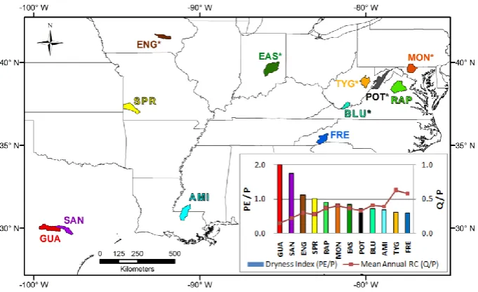
Figure 3: Location of study sites and their aridity index and runoff coefficient for the period 1990-1999. Snow catchments are indicated with an *.
Fig. 3. Location of study sites and their aridity index and runoff coefficient for the period 1990–1999. Snow catchments are indicated with an∗.
Nash-Sutcliffe efficiency (Nash and Sutcliffe, 1970) measure for streamflow values.
3.2 Matching hydrologic signatures
The final step in our model identification procedure is to compare modeled and observed hydrologic signatures, such as the annual runoff coefficient, annual baseflow index and the slope of the flow duration curve (Gupta et al., 2008; Yil-maz et al., 2008). The annual runoff coefficient for any given hydrologic year is defined as:
RQP = 365 X
t=1 Q(t )
P (t ) (35)
wheretis day in hydrologic year (1 October–30 September). Similarly, the annual baseflow index is defined as:
IBF = 365 X
t=1 Qb(t )
Q(t ) . (36)
The slope of the flow duration curve is defined as (Yadav et al., 2007; Sawicz et al., 2011):
SFDC =
ln (Q33%) − ln(Q66%)
0.66−0.33 (37)
whereQ33% andQ66% are the flow values exceeded 33 % and 66 % of the time, respectively. Discrepancies between modeled and observed hydrologic signatures are used to re-peat the parameter estimation procedure after Step 1 until no further improvements in reproducing these signatures are obtained.
4 Study sites and model identification results
4.1 Study sites across climate gradient
We applied the above described hydrologic analysis proce-dure to 12 MOPEX catchment east of the Rocky Moun-tains, USA. These catchments were previously used in van Werkhoven et al. (2008) to study SAC-SMA (Sacramento Soil Moisture Accounting) model parameter sensitivities across a hydroclimate gradient using multiple time periods between 1980–1989.
As can be seen from the listed wetness indices and runoff coefficients in Fig. 3, these catchments represent a wide range of climate and hydrologic regimes. Table 1 lists some catchment characteristics of our 12 study sites. Catchment area ranges from 1000 km2 to 4500 km2. Mean catchment elevation ranges from about 100 to 800 m a.s.l. The mean annual precipitation ranges from 750 mm to 1500 mm, and the mean annual potential evapotranspiration ranges from 1500 mm to 700 mm.
4.2 Forcing data and a priori parameter assignments
4.2.1 Forcing data
The model uses the following eight variables as input time series: precipitation, land surface albedo, air tem-perature, long and short wave downward radiation, atmo-spheric pressure, actual vapor pressure and wind speed. Daily precipitation data is provided through the MOPEX website (ftp://hydrology.nws.noaa.gov/pub/gcip/mopex/US Data/) (Duan et al., 2006). The other seven variables are derived from the 3-h, 1/8 degree hydroclimate data set de-veloped by Maurer et al. (2002), and available at http://
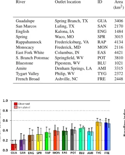
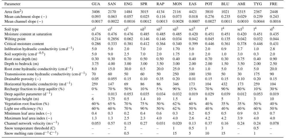
[image:10.595.128.469.61.269.2]Table 1. Watershed characteristics.
River Outlet location ID Area Mean Mean Mean Mean
(km2) Elevation AnnualP Annual PE Annual RC
(m) (mm) (mm) (Q/P)
Guadalupe Spring Branch, TX GUA 3406 542 765 1528 0.15
San Marcos Luling, TX SAN 2170 295 827 1449 0.22
English Kalona, IA ENG 1484 254 893 994 0.30
Spring Waco, MO SPR 3015 329 1076 1094 0.28
Rappahannock Fredericksburg, VA RAP 4134 204 1030 920 0.37
Monocacy Frederick, MD MON 2116 194 1041 896 0.40
East Fork White Columbus, IN EAS 4421 268 1015 855 0.37
S. Branch Potomac Springfield, WV POT 3810 651 1042 761 0.33
Bluestone Pipestem, WV BLU 1021 787 1018 741 0.41
Amite Denham Springs, LA AMI 3315 77 1564 1073 0.39
Tygart Valley Philip, WV TYG 2372 709 1166 711 0.63
French Broad Ashville, NC FRE 2448 819 1383 819 0.58
[image:11.595.54.313.88.410.2]50
Figure 4: Observed versus simulated runoff coefficients for all 12 catchments for the period 1990-1999. The error bars represent ± one standard deviation of the observed and modeled annual
runoff coefficients, respectively.
Fig. 4. Observed versus simulated runoff coefficients for all 12 catchments for the period 1990–1999. The error bars represent±1 standard deviation of the observed and modeled annual runoff coef-ficients, respectively.
www.hydro.washington.edu. The 3-h data are converted to daily averages and then spatially averaged over the catch-ments using a weighted averaging procedure that accounts for complete or partial coverage of data grid and catchment boundaries.
4.2.2 A priori parameter assignments
For each basin, the MOPEX database provides fractional spatial coverage of each of the 16 USDA soil types, as well as the fractional spatial coverage of vegetation type ac-cording to the University of Maryland vegetation classifi-cation system (see also http://www.geog.umd.edu/landcover/ global-cover.html). From this information, the dominant soil type and vegetation type is selected and typical parameter values are selected from Clapp and Hornberger (1978) for to-tal soil porosity, and from the North American Land Data As-similation System – NLDAS (http://ldas.gsfc.nasa.gov/nldas/ NLDASmapveg.php) database for initial values of root zone depth and vegetation height.
[image:11.595.48.287.293.410.2]51
Figure 5: Observed versus simulated baseflow indices for all 12 catchments for the period 1990-1999. The error bars represent ± one standard deviation of the observed and modeled annual
baseflow indices, respectively.
Fig. 5. Observed versus simulated baseflow indices for all 12 catch-ments for the period 1990–1999. The error bars represent±1 stan-dard deviation of the observed and modeled annual baseflow in-dices, respectively.
4.3 Modeling results
[image:11.595.310.546.293.411.2]3422 G. Carrillo et al.: Hydrological analysis of catchment behavior through process-based modeling
52
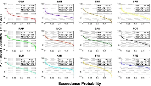
Figure 6
: Observed (solid line) versus simulated (dashed line) flow duration curves for all 12
catchments for the period 1990-1999. The inset shows the Nash-Sutcliffe efficiency (NSE), the
Nash-Sutcliffe efficiency after log-transforming streamflow (NSE-Log) and the mean absolute
error between observed and modeled ordinates of the FDC (Mean AE; in mm/d).
Fig. 6. Observed (solid line) versus simulated (dashed line) flow duration curves for all 12 catchments for the period 1990–1999. The inset shows the Nash-Sutcliffe efficiency (NSE), the Nash-Sutcliffe efficiency after log-transforming streamflow (NSE-Log) and the mean absolute error between observed and modeled ordinates of the FDC (Mean AE; in mm d−1).
In order to evaluate the model performance at daily time steps, Fig. 6 shows the observed and modeled flow duration curves for the period 1990–1999 for all catchments. Even though the model efficiency to reproduce observed hydro-graphs is moderate (see inset values of Nash-Sutcliffe effi-ciencies in Fig. 6), the match with observed flow duration curves is remarkable at all flow levels (with a few excep-tions). This suggests that the model captures the dynamic transformation of climate forcing into streamflow rather well but that timing of individual storm events may not be mod-eled accurately. For the purpose of this study we consider it more important to be able to reproduce the different modes of response (in terms of frequencies of low, medium and high flow) given certain climate forcing than to match/over-parameterize the model to fit hydrographs.
Figure 7 compares the monthly regime curves of precipi-tation, evapotranspiration and discharge for two catchments in different climate settings. San Marcos catchment in Texas (left panel of Fig. 7) is a water-limited catchment, whereas Amite catchment in Louisiana (right panel of Fig. 7) is a more energy-limited catchment. The model reproduces the discharge regime curve for both catchments remarkably well, illustrating that the model is capable of filtering different climate signals in ways that are comparable with the real catchment filters. Similar results were obtained for the other 10 catchments (not shown).
5 Discussion
5.1 Model parameters and time scales
Table 2 lists all model parameters for all 12 catchments, to-gether with catchment characteristics derived from available geographic information, such as drainage area, mean catch-ment slope and mean channel slope. Total porosity was se-lected from look-up tables (Clapp and Hornberger, 1978) based on dominant soil type. All other parameters were ob-tained using the methods described in Sect. 3. From these model parameters we have computed the different time scales discussed in Sect. 2.4 (see Table 3). Many different dimen-sionless numbers can now be formulated as ratios of time scales. In the next section we relate these time scales and di-mensionless numbers to hydrologic signatures to reveal scal-ing relationships that could be used to determine hydrologic similarity between different catchments.
An attempt to perform an automated parameter sensitivity analysis failed due to the highly coupled and non-linear char-acter of the model equations, which caused instabilities in the numerical solution of Eq. (1). In future work we will refor-mulate the presented model and replace the dynamic ground-water equation with derived storage-discharge relationships. This will remove most of the issues of numerical stability and will allow testing of the parameter uncertainty and sensitivity
[image:12.595.59.540.63.337.2]53
Figure 7: Observed and simulated regime curves of monthly precipitation, evapotranspiration and discharge. Potential evapotranspiration is computed from the model using minimal stomatal resistance. – Left = San Marcos,TX – Right = Amite, LA – Vertical lines are ± one standard deviation.
Fig. 7. Observed and simulated regime curves of monthly precipita-tion, evapotranspiration and discharge. Potential evapotranspiration is computed from the model using minimal stomatal resistance. – Left panel = San Marcos, TX – Right panel = Amite, LA – Vertical lines are±1 standard deviation.
required to assess how representative the listed parameter values in Table 2 are.
5.2 Regionalization and scaling relationships
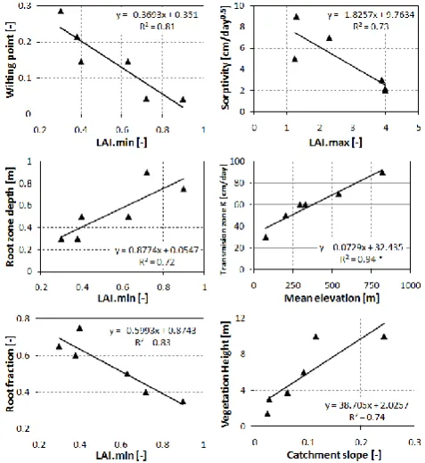
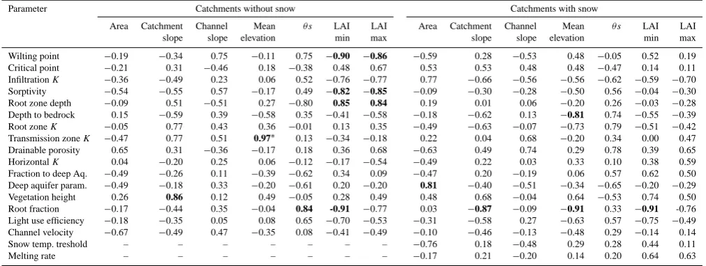
We regressed all readily available catchment characteristics, such as drainage area and mean catchment slope, to the dif-ferent model parameters, in an attempt to reveal regionaliza-tion patterns. Not many linear regressions between catch-ment characteristics and model parameters were statistically significant at 95 % confidence limits. Table 4 shows all regression relationships that were significant withp <0.05 (some were significant atp <0.01, indicated by∗). Figure 8 shows some of these statistically significant relationships for the no-snow dominated catchments. Only very few signifi-cant relationships showed up for all 12 catchments or for the 6 snow dominated catchments, indicating that the parameters of the snow dominated catchments were not related to catch-ment characteristics and therefore could not be regionalized. The remaining regression relations for the 6 no-snow catch-ments appear to be rather strong. In particular, information of minimum and maximum LAI can be translated to root zone and vegetation parameters in the model quite reliably. Mean elevation of the 6 catchments seems to be strongly related to the saturated hydraulic conductivity of the transmission zone,
[image:13.595.50.285.60.329.2]54
Figure 8: Significant (p<0.05; * indicates p<0.01) linear regression relationships between catchment characteristics (minimum and maximum LAI, mean elevation and mean catchment
slope) and different model parameters for 6 no-snow dominated catchments.
Fig. 8. Significant (p <0.05; ∗indicatesp <0.01) linear regres-sion relationships between catchment characteristics (minimum and maximum LAI, mean elevation and mean catchment slope) and dif-ferent model parameters for 6 no-snow dominated catchments.
while catchment slope defines vegetation height. The latter relationship is most likely caused by the a priori choice of vegetation height from land cover databases that show a sim-ilar relation between vegetation height and catchment slope (K. Sawicz, personal communication, 2010). However, these regressions are mainly the result of our hydrograph analy-sis to inform model parameters rather than from regression catchment characteristics and hydrologic response. Obvi-ously more work is needed to define the robustness of these relationships, their physical meaning (why is hydraulic con-ductivity of the transmission zone related to mean eleva-tion?), as well as answering the question why no significant relationships showed up for the snow dominated catchments. It is possible that the soil parameters defined during the dor-mant season are affected during the snow accumulation pe-riod while in fact most partitioning processes controlled by these soil parameters are inactive. Another possible explana-tion is that different parameters of the model control differ-ent runoff generation mechanisms in differdiffer-ent climates (van Werkhoven et al., 2008). We will address this issue in our on-going research.
[image:13.595.308.547.63.323.2]3424 G. Carrillo et al.: Hydrological analysis of catchment behavior through process-based modeling
[image:14.595.50.284.61.329.2]55
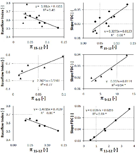
Figure 9: Linear and non-linear regression relationships, significant at p<0.05 (* indicates p<0.01), between hydrologic signatures and model time scales. Triangles indicate no snow
catchments and dots represent snow catchments.
Fig. 9. Linear and non-linear regression relationships, significant at p <0.05 (∗indicatesp <0.01), between hydrologic signatures and model time scales. Triangles indicate no snow catchments and dots represent snow catchments.
regression functions were altered when non-linear relations were apparent from the data trends. Again, no strong regres-sion relationships showed up for the snow-dominated catch-ments, so Fig. 9 shows only significant relationships for no snow catchments. It should be kept in mind that the reported R2values apply to the initial linear regression analysis (as well as the significance levels), even though after inspection of the data trends it was clear that non-linear (power law) regressions better represent the patterns. The runoff coeffi-cient is related to 3 time scales of the models: the time scale related to emptying the canopy store (function of potential evaporation, and thus strongly related to climate), the time scale associated with emptying the root zone by transpira-tion (a functranspira-tion of actual evapotranspiratranspira-tion and thus part of the competition between ET and drainage), the time scale related to emptying the transmission zone through drainage (clearly defining the generation of slow flow at the expense of ET). RC is clearly also affected by the mean storm dura-tion, a climate time scale and not a model time scale. Zoom-ing in on the latter two model time scales and how they re-late to RC, it is interesting to note that RC increases when it takes longer for the root zone to be emptied by ET, indicat-ing that in such situations water can move through the root zone to become baseflow or is more likely to generate quick flow. Likewise, RC is higher when it takes less time to empty the transmission zone through drainage, indicating the (lack
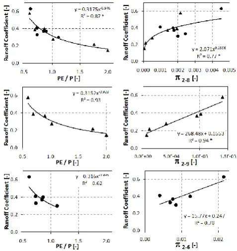
[image:14.595.307.546.62.315.2]56
Figure 10: Significant linear and non-linear regression relations between the runoff coefficient and different dimensionless numbers: Left: aridity index; Right: three dimensionless numbers
related to different time scales in the models (2: canopy emptying; 6: root zone emptying by drainage; 8: transmission zone filling; 9: transmission zone emptying). Triangles indicate no-snow
catchments and dots represent snow catchments.
Fig. 10. Significant linear and non-linear regression relations be-tween the runoff coefficient and different dimensionless numbers: left panel: aridity index; right panel: three dimensionless numbers related to different time scales in the models (2: canopy emptying; 6: root zone emptying by drainage; 8: transmission zone filling; 9: transmission zone emptying). Triangles indicate no-snow catch-ments and dots represent snow catchcatch-ments.
of) feedback between subsurface moisture storage and ET through capillary fluxes.
Baseflow index is strongly and linearly related to the time scale associated with filling up the root zone by rainfall. When that time scale is short, less water will leave the catch-ment as baseflow and more as surface runoff. This does not seem to be affected much by climate, since even in our most arid catchments the baseflow index can be high (e.g. GUA which is a karst dominated catchment).
The only relationship that holds for all 12 catchments is between the slope of the FDC and the time scale of the deep aquifer. This relationship is especially robust because of the physical link between short time scales of the linear reser-voir behavior and the release of water from the catchment, as captured by the slope of the FDC.
Finally, we regressed hydrologic signatures with different dimensionless numbers, created as ratios of the model time scales. We usedπi-j to indicate the dimensionless number
created by time scaleiover time scalej, withiandjindices referring to time scales listed in Table 3. For instance,π2-8 is defined by the ratio of the time scale to empty canopy stor-age by potential ET and the time scale of the perched aquifer advection. It is clear from Fig. 10 that the aridity index is a strong control on the runoff coefficient, for all 12 catchments
Table 2. Model parameters.
Parameter GUA SAN ENG SPR RAP MON EAS POT BLU AMI TYG FRE
Area (km2) 3406 2170 1484 3015 4134 2116 4421 3810 1021 3315 2367 2448 Mean catchment slope (−) 0.093 0.063 0.057 0.025 0.116 0.073 0.018 0.276 0.235 0.029 0.239 0.243 Mean channel slope (−) 0.0017 0.0022 0.0016 0.0012 0.0013 0.0028 0.0007 0.0027 0.0011 0.0010 0.0044 0.0016 Soil type cl1 cl1 cl1 sil2 sil2 sil2 scl3 l4 l4 scl3 l4 sl5 Moisture content at saturation 0.476 0.476 0.476 0.485 0.485 0.485 0.420 0.451 0.451 0.420 0.451 0.435 Wilting point 0.214 0.2856 0.062 0.146 0.146 0.034 0.042 0.045 0.135 0.042 0.032 0.044 Critical moisture content 0.286 0.333 0.381 0.412 0.364 0.340 0.399 0.446 0.361 0.378 0.446 0.431 Infiltration hydraulic conductivity (cm d−1) 5.0 5.0 2.0 7.0 2.0 1.70 5.0 2.0 0.9 2.7 1.0 2.8
Soil sorptivity (cm d−0.5) 5.0 9.0 2.5 7.0 2.0 1.75 1.0 2.0 1.0 3.0 0.3 2.0 Root zone depth (m) 0.30 0.30 0.70 0.50 0.50 0.40 0.40 0.70 0.30 0.75 0.40 0.90 Depth to bedrock (m) 3.75 4.00 3.00 3.00 3.50 3.00 2.00 2.00 1.50 3.50 2.00 2.50 Root zone hydraulic conductivity (cm d−1) 8.0 15.0 30.0 0.5 20.0 25.0 5.0 1.0 5.0 5.0 5.0 20.0 Transmission zone hydraulic conductivity (cm d−1) 70 60 50 60 50 250 100 150 50 30 175 90
Drainable porosity (−) 0.05 0.055 0.15 0.10 0.35 0.20 0.01 0.15 0.15 0.10 0.20 0.15 Horizontal hydraulic conductivity (m d−1) 259 147 69 86 86 346 173 104 432 173 259 104
Recharge fraction to deep aquifer (%) 0 % 70 % 50 % 10 % 5 % 90 % 15 % 70 % 90 % 80 % 10 % 30 % Deep aquifer parameter (d−1) – 0.013 0.053 0.035 0.034 0.032 0.019 0.029 0.039 0.012 0.053 0.019
Vegetation height (m) 6 3.75 0.5 1.4 10 1.5 4 8 5 3 3 10
Vegetation root fraction (%) 60 % 65 % 70 % 75 % 50 % 62 % 60 % 40 % 35 % 35 % 50 % 40 % Light use efficiency (%) 60 % 60 % 70 % 90 % 50 % 62 % 50 % 40 % 40 % 40 % 60 % 50 % Minimum leaf area index (−) 0.4 0.3 0.2 0.4 0.6 0.3 0.2 0.5 0.5 0.9 0.3 0.7 Maximum leaf area index (−) 1.3 1.3 2.5 2.3 4.0 4.0 2.6 4.2 4.2 3.9 4.0 4.0 Channel network velocity (m s−1) 0.053 0.57 0.15 0.27 0.031 0.020 0.13 0.37 0.16 0.24 0.24 0.078
Snow temperature threshold (C) – – 2 – – 1 0.5 1 3 – 0.5 –
Snow melting rate (mm d−1C−1) – – 0.5 – – 15 5 10 15 – 1 –
1cl = clay;2sil = silt;3scl = sandy clay;4l = loam;5sl = sandy loam
(but somehow more strong for the no-snow catchments). This is no surprise since the left panels of Fig. 10 are nothing but the Budyko curve for our catchments. However, for the no-snow catchments, a dimensionless number defined by the time scale to empty the canopy storage (linked to PET) and the diffusion time scale of perched aquifer drainage (linked to catchment early-stage drainage), does equally well to ex-plain the observed variance compared to the aridity index (R2 of 0.935 atp <0.01 vs. 0.926 atp <0.05, respectively).
Figure 11 suggests that the same dimensionless number (π15-12: ratio of interstorm duration to deep aquifer time constant) explains both the baseflow index and the slope of the FDC for all 12 catchments, even though stronger rela-tionships are possible when separating snow from no-snow catchments and when using different dimensionless num-bers. In any case, the time scales of aquifer drainage always play an important role to explain these hydrologic signatures, indicating that subsurface catchment characteristics are con-trolling release of water stored in the saturated zone.
5.3 Co-variation of climate, vegetation and soil time scales
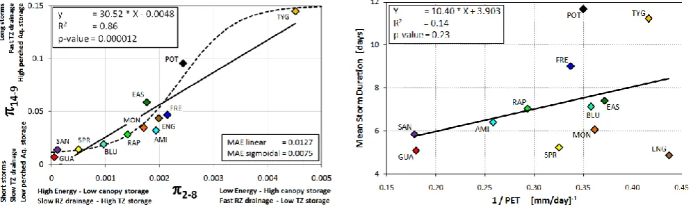
Finally, we investigated how different ratios of time scales are related to each other. If significant (linear or non-linear) relationships exist between different dimensionless numbers characterizing the catchments, this could indicate that dif-ferent time scales interact to create systematic emerging patterns of hydrologic partitioning across the climate gradi-ent. For example, Fig. 12 shows a strong linear relationship
(R2= 0.86;p <0.0001) betweenπ14-9andπ2-8. Catchments with low values of these two dimensionless numbers have cli-mates characterized by high PET and short storm durations, have low canopy storage capacity (low LAI), slowly drain the root zone and transmission zone, and have low perched aquifer storage capacity and hence high transmission zone storage capacity. The opposite is true for catchments with high values for these 2 dimensionless numbers. The data suggest either a linear trend between those two extremes or a non-linear (sigmoid) trend. The latter has a lower mean abso-lute error regarding the data points. All this indicates that cli-mate, vegetation and subsurface characteristics of root zone, transmission zone and perched aquifer somehow co-evolve along the climate gradient.
3426 G. Carrillo et al.: Hydrological analysis of catchment behavior through process-based modeling
Table 3. Time scales.
No. Time Scale (days) GUA SAN ENG SPR RAP MON EAS POT BLU AMI TYG FRE
1 Canopy filling 0.07 0.07 0.12 0.10 0.19 0.19 0.14 0.29 0.24 0.12 0.19 0.15
2 Canopy emptying 0.04 0.05 0.22 0.15 0.23 0.29 0.19 0.29 0.30 0.20 0.33 0.27
3 Snow melting – – 22.7 – – 19.6 26.7 33.7 8.0 – 20.7 –
4 Root zone filling by 13.1 12.5 22.7 5.5 15.3 15.3 3.8 13.5 9.7 2.3 8.9 18.9
rainfall
5 Root zone filling by – – 43.6 – – 41.2 23.1 50.7 7.6 – 19.7 –
melting
6 Root zone emptying by 59.5 31.6 25.9 62.1 35.4 23.4 25.2 42.8 75.2 42.6 15.5 69.4
drainage
7 Root zone emptying by 20.6 21.4 53.8 45.0 48.6 42.8 20.0 76.1 31.7 23.8 40.9 94.5
transpiration
8 Transmission zone 833 411 110 298 167 169 108 121 310 104 74 125
filling
9 Transmission zone 742 424 112 370 248 175 126 122 372 198 77 193
emptying
10 Boussinesq aquifer 0.8 1.3 9.3 25.8 13.6 2.1 11.2 1.5 0.8 4.6 0.9 1.5
advective
11 Boussinesq aquifer 9.4 6.7 68.4 141.4 198.3 17.1 44.4 59.2 65.6 15.0 31.5 37.7
diffusion
12 Deep aquifer – 80.0 18.8 28.6 29.4 31.3 52.6 34.5 25.6 83.3 18.9 52.6
13 Channel flow 2.7 2.0 4.2 2.8 3.0 3.0 6.9 4.3 4.0 4.1 3.3 9.1
14 Mean Storm Duration 5.09 5.85 4.88 5.24 7.05 6.06 7.41 11.68 7.14 6.40 11.24 9.02
15 Mean InterStorm 2.86 2.88 2.49 2.43 2.24 2.17 1.91 1.70 1.99 2.44 1.76 2.11
Duration
Table 4. Linear correlation coefficients between catchment characteristics and model parameters.
Parameter Catchments without snow Catchments with snow
Area Catchment Channel Mean θ s LAI LAI Area Catchment Channel Mean θ s LAI LAI slope slope elevation min max slope slope elevation min max
Wilting point −0.19 −0.34 0.75 −0.11 0.75 −0.90 −0.86 −0.59 0.28 −0.53 0.48 −0.05 0.52 0.19 Critical point −0.21 0.31 −0.46 0.18 −0.38 0.48 0.67 0.53 0.53 0.48 0.48 −0.47 0.14 0.11 InfiltrationK −0.36 −0.49 0.23 0.06 0.52 −0.76 −0.77 0.77 −0.66 −0.56 −0.56 −0.62 −0.59 −0.70 Sorptivity −0.54 −0.55 0.57 −0.17 0.49 −0.82 −0.85 −0.09 −0.30 −0.28 −0.50 0.56 −0.04 −0.30 Root zone depth −0.09 0.51 −0.51 0.27 −0.80 0.85 0.84 0.19 0.01 0.06 −0.20 0.26 −0.03 −0.28 Depth to bedrock 0.15 −0.59 0.39 −0.58 0.35 −0.41 −0.58 −0.18 −0.62 0.13 −0.81 0.74 −0.55 −0.39 Root zoneK −0.05 0.77 0.43 0.36 −0.01 0.13 0.35 −0.49 −0.63 −0.07 −0.73 0.79 −0.51 −0.42 Transmission zoneK −0.47 0.77 0.51 0.97∗ 0.13 −0.34 −0.18 0.22 0.04 0.68 −0.20 0.34 0.00 0.47 Drainable porosity 0.65 0.31 −0.36 −0.17 0.18 0.36 0.68 −0.63 0.49 0.74 0.29 0.78 0.39 0.65 HorizontalK 0.04 −0.20 0.25 0.06 −0.12 −0.17 −0.54 −0.49 0.22 0.03 0.33 0.10 0.38 0.59 Fraction to deep Aq. −0.49 −0.26 0.11 −0.39 −0.62 0.34 0.09 −0.47 0.20 −0.19 0.06 0.57 0.62 0.50 Deep aquifer param. −0.49 −0.18 0.33 −0.20 −0.61 0.20 −0.20 0.81 −0.40 −0.51 −0.34 −0.65 −0.20 −0.29 Vegetation height 0.26 0.86 0.12 0.49 −0.05 0.28 0.49 0.48 0.68 −0.04 0.64 −0.53 0.74 0.50 Root fraction −0.17 −0.44 0.35 −0.04 0.84 -0.91 −0.77 0.03 −0.87 −0.09 −0.91 0.33 −0.91 -0.76 Light use efficiency −0.18 −0.35 0.05 0.08 0.65 −0.70 −0.53 −0.31 −0.58 0.27 −0.63 0.57 −0.75 −0.49 Channel velocity −0.67 −0.49 0.47 −0.35 0.08 −0.41 −0.49 −0.10 −0.46 −0.13 −0.48 0.29 −0.14 0.14 Snow temp. treshold – – – – – – – −0.76 0.18 −0.48 0.29 0.28 0.44 0.11
Melting rate – – – – – – – −0.17 0.21 −0.20 0.14 0.20 0.64 0.63
Bold prints are significant at 95 % CL;∗indicates significance at 99 % CL.
[image:16.595.47.553.474.665.2]Table 5. Linear correlation coefficients between hydrologic signatures and model time scales.
Time Scale Runoff coefficient Baseflow index Slope FDC
All No-Snow Snow All No-Snow Snow All No-Snow Snow
Canopy filling 0.46 0.72 0.03 0.08 0.34 0.49 0.26 −0.31 −0.19
Canopy emptying 0.80∗ 0.92∗ 0.65 −0.02 0.31 0.07 0.25 −0.38 −0.12
Snow melting −0.29 – −0.29 0.47 – 0.47 −0.28 – −0.28
Root zone filling by rainfall −0.01 0.29 −0.44 0.30 0.87 −0.49 0.21 −0.26 0.60
Root zone filling by melting −0.54 – −0.54 0.23 – 0.23 −0.03 – −0.03
Root zone emptying by drainage −0.11 0.30 −0.27 0.18 0.11 0.00 −0.07 0.28 0.29
Root zone emptying by transpiration 0.45 0.85 −0.30 0.45 0.65 0.09 −0.02 −0.29 0.22
Transmission zone filling −0.68 −0.81 −0.17 0.01 −0.17 −0.04 −0.03 0.51 0.15
Transmission zone emptying −0.66 −0.84 −0.14 0.02 −0.23 −0.06 −0.11 0.57 0.16
Boussinesq aquifer advective −0.23 −0.06 −0.48 −0.38 −0.59 −0.18 0.17 0.69 0.15
Boussinesq aquifer diffusion −0.03 0.13 −0.53 −0.15 −0.21 −0.43 0.19 0.44 0.78
Deep aquifer −0.23 −0.09 −0.34 0.39 0.11 0.73 −0.77∗ −0.72 −0.65
Channel flow −0.18 −0.18 −0.08 0.25 0.12 0.40 −0.22 0.26 −0.57
Mean Storm Duration 0.65 0.94∗ 0.50 0.33 0.80 0.42 −0.05 −0.71 −0.31
Mean InterStorm Duration −0.70 −0.89 −0.47 −0.07 −0.29 −0.62 −0.22 0.24 0.54
Bold prints are significant at 95 % CL;∗indicates significance at 99 % CL.
57
Figure 11: Significant linear relationships between baseflow index and slope of the FDC and different dimensionless numbers related to model time scales (4: root zone filling by rain; 9: transmission zone emptying; 11: Boussinesq aquifer diffusion; 12: deep aquifer; 15: mean
inter-storm duration). Triangles indicate no snow catchments and dots represent snow catchments.
Fig. 11. Significant linear relationships between baseflow index and slope of the FDC and different dimensionless numbers related to model time scales (4: root zone filling by rain; 9: transmission zone emptying; 11: Boussinesq aquifer diffusion; 12: deep aquifer; 15: mean inter-storm duration). Triangles indicate no snow catch-ments and dots represent snow catchcatch-ments.
Apparently, our hydrograph analysis with the aid of the process-based model resulted in a systematic variation of subsurface properties, expressed as time scales related to the root zone and transmission zone, between dry less vegetated and wet more vegetated catchments. At the far left in Fig. 12 appear the catchments situated in Texas (GUA and SAN) and Missouri (SPR) and at the far right are catchments situated in West Virginia (POT and TYG). If such relationship between climate, vegetation and soil time scales can be shown to hold for other catchments along similar climate gradients, it can provide guidance for catchment model parameterization that would apply to ungauged basins. Obviously more research is required to support this conclusion.
5.4 Limitation of bottom-up modeling approach to
explain hydrologic similarity
[image:17.595.49.286.325.591.2]