Hydrol. Earth Syst. Sci., 17, 3005–3021, 2013 www.hydrol-earth-syst-sci.net/17/3005/2013/ doi:10.5194/hess-17-3005-2013
© Author(s) 2013. CC Attribution 3.0 License.
EGU Journal Logos (RGB)
Advances in
Geosciences
Open Access
Natural Hazards
and Earth System
Sciences
Open Access
Annales
Geophysicae
Open Access
Nonlinear Processes
in Geophysics
Open Access
Atmospheric
Chemistry
and Physics
Open Access
Atmospheric
Chemistry
and Physics
Open Access
Discussions
Atmospheric
Measurement
Techniques
Open Access
Atmospheric
Measurement
Techniques
Open Access
Discussions
Biogeosciences
Open Access Open Access
Biogeosciences
Discussions
Climate
of the Past
Open Access Open Access
Climate
of the Past
Discussions
Earth System
Dynamics
Open Access Open Access
Earth System
Dynamics
Discussions
Geoscientific
Instrumentation
Methods and
Data Systems
Open Access
Geoscientific
Instrumentation
Methods and
Data Systems
Open Access
Discussions
Geoscientific
Model Development
Open Access Open Access
Geoscientific
Model Development
DiscussionsHydrology and
Earth System
Sciences
Open Access
Hydrology and
Earth System
Sciences
Open Access
Discussions
Ocean Science
Open Access Open Access
Ocean Science
DiscussionsSolid Earth
Open Access Open Access
Solid Earth
Discussions
The Cryosphere
Open Access Open Access
The Cryosphere
DiscussionsNatural Hazards
and Earth System
Sciences
Open Access
Discussions
Statistical modelling of the snow depth distribution
in open alpine terrain
T. Gr ¨unewald1,2, J. St¨otter3, J. W. Pomeroy4, R. Dadic5,6, I. Moreno Ba ˜nos7, J. Marturi`a7, M. Spross3, C. Hopkinson8, P. Burlando5, and M. Lehning1,2
1WSL Institute for Snow and Avalanche Research SLF, Fl¨uelastrasse 35, 7260 Davos, Switzerland
2Cryos, School of Architecture, Civil and Environmental Engineering, ´Ecole Polytechnique F´ed´erale de Lausanne,
GRAO 402 – Station 2, 1015 Lausanne, Switzerland
3Institute of Geography, University of Innsbruck, Innrain 52, 6020 Innsbruck, Austria
4Centre for Hydrology, University of Saskatchewan, 117 Science Place, Saskatoon, Saskatchewan, S7N 5C8, Canada 5Institute of Environmental Engineering, ETH Zurich, 8093 Zurich, Switzerland
6Antarctic Research Centre, Victoria University of Wellington, P.O. Box 600, Wellington, New Zealand 7Institut Geol`ogic de Catalunya, C/Balmes 209–211, 08006 Barcelona, Spain
8Department of Geography, University of Lethbridge, 4401 University Drive West, Lethbridge, Alberta, T1K 3M4, Canada
Correspondence to: T. Gr¨unewald ([email protected])
Received: 28 February 2013 – Published in Hydrol. Earth Syst. Sci. Discuss.: 13 March 2013 Revised: 11 June 2013 – Accepted: 26 June 2013 – Published: 1 August 2013
Abstract. The spatial distribution of alpine snow covers is
characterised by large variability. Taking this variability into account is important for many tasks including hydrology, glaciology, ecology or natural hazards. Statistical modelling is frequently applied to assess the spatial variability of the snow cover. For this study, we assembled seven data sets of high-resolution snow-depth measurements from different mountain regions around the world. All data were obtained from airborne laser scanning near the time of maximum sea-sonal snow accumulation. Topographic parameters were used to model the snow depth distribution on the catchment-scale by applying multiple linear regressions. We found that by av-eraging out the substantial spatial heterogeneity at the metre scales, i.e. individual drifts and aggregating snow accumula-tion at the landscape or hydrological response unit scale (cell size 400 m), that 30 to 91 % of the snow depth variability can be explained by models that are calibrated to local conditions at the single study areas. As all sites were sparsely vegetated, only a few topographic variables were included as explana-tory variables, including elevation, slope, the deviation of the aspect from north (northing), and a wind sheltering parame-ter. In most cases, elevation, slope and northing are very good predictors of snow distribution. A comparison of the models showed that importance of parameters and their coefficients
differed among the catchments. A “global” model, combin-ing all the data from all areas investigated, could only explain 23 % of the variability. It appears that local statistical models cannot be transferred to different regions. However, models developed on one peak snow season are good predictors for other peak snow seasons.
1 Introduction
human activities, including agriculture (e.g. irrigation), hy-dropower or water resources management, depend on in-formation on the spatio-temporal variability of snow cover and melt. In order to capture the temporally varying run-off caused by snowmelt, hydrological models need to account for the spatial distribution of snow.
Recent years have seen advances in modelling snow dis-tributions by applying sophisticated physically based snow cover redistribution models (Pomeroy and Li, 2000; Liston and Elder, 2006; Lehning et al., 2008; Schneiderbauer and Prokop, 2011). Such models have been operated at grid res-olutions of a few metres (e.g. Essery et al., 1999; Liston and Elder, 2006; Mott and Lehning, 2010; Mott et al., 2010; Schneiderbauer and Prokop, 2011) to hundreds of meters (e.g. Bernhardt et al., 2009; Bavay et al., 2009, 2013; MacDonald et al., 2010; Magnusson et al., 2010). These models require high level input, including meteorolog-ical data, sometimes detailed flow fields (Raderschall et al., 2008) and sometimes high-resolution digital elevation mod-els. They are therefore very expensive in terms of required information and calculation resources, and have not been ap-plied for larger areas or longer time frames. In general, there is a trade-off between model complexity and generality on the one hand and computation time on the other hand al-though reasonable compromises have been achieved using the hydrological response unit concept (MacDonald et al., 2009; Fang and Pomeroy, 2009) which derives from that of landscape units for stratified snow sampling (e.g. Steppuhn and Dyck, 1974).
Topography strongly influences snow distribution but is not a causative factor in itself (e.g. McKay and Gray, 1981; Pomeroy and Gray, 1995). The spatial heterogeneity of the snow cover is attributed to a number of different processes which act on different scales: local precipitation amounts are strongly affected by the interaction of the terrain with the lo-cal weather and climate (Choularton and Perry , 1986; Daly et al., 1994; Beniston et al., 2003; Mott et al., 2013). Wind plays a major role for the deposition and redistribution of snow (e.g. McKay and Gray, 1981; Pomeroy and Gray, 1995; Essery et al., 1999; Trujillo et al., 2007; Lehning et al., 2008). Moreover, snow can be relocated by avalanches and slough-ing (Bl¨oschl and Kirnbauer, 1992; Gruber, 2007; Bernhardt and Schulz, 2010), and the local radiation and energy bal-ance influence the spatially varying ablation processes (Cline et al., 1998; Pomeroy et al., 1998, 2004; Pohl et al., 2006; Mott et al., 2011).
Many studies have attempted to exploit the relationship between topography and snow in statistical models. Topo-graphic parameters serve as explanatory variables for ex-plaining the spatial heterogeneity of snow depth, snow wa-ter equivalent (SWE) or melt rates. Several studies have successfully developed binary regression tree models (e.g. Elder et al., 1998; Balk and Elder, 2000; Erxleben et al., 2002; Winstral et al., 2002; Anderton et al., 2004; Molotch et al., 2005; Lopez-Moreno and Nogues-Bravo, 2006; Litaor
et al., 2008), where the response data (e.g. snow depth) are repeatedly split along a predictor (e.g. terrain parameter) into sub-groups by minimising the sum of the residuals. Such re-gression tree models were capable of explaining 18 to 90 % of the snow-cover variability. The performance of the models depends on both the complexity of the tree (number of ex-planatory parameters and number of splits), and on the qual-ity and complexqual-ity of the data that are analyzed.
A second very common statistical approach is multiple lin-ear regression. As in the regression tree models, terrain pa-rameters serve as explanatory variables. An early example is the multivariate regression model developed by Golding (1974) and applied to Marmot Creek Research Basin, Al-berta. Golding (1974) found that elevation, topographic po-sition, aspect, slope, and forest density were the most impor-tant variables for predicting snow accumulation but together these could only explain 48 % of the variation of SWE. Based on 106 snow poles Lopez-Moreno and Nogues-Bravo (2006) were able to explain more than 50 % of the large scale snow depth variability over the Pyrenees with elevation, elevation range, radiation and two location parameters. Chang and Li (2000) used monthly SWE data averaged from 13 to 36 snow courses in Idaho to build regression models with a combina-tion of elevacombina-tion, slope, aspect and a relative posicombina-tion. The models could explain 60 to 90 % of the monthly SWE vari-ability for different regions and large catchments. Marchand and Killingtveit (2005) found that it was possible to model snow depth in open and forested areas of a large (849 km2) Norwegian catchment with different measures of elevation, aspect, curvature and slope (R2= 5–48 %). For their anal-ysis, they aggregated a very large number of snow depth measurements, obtained by georadar and hand probing to a grid of 1000 m. Pomeroy et al. (2002) used a paramet-ric model derived from a physically based snow intercep-tion model to explain snow accumulaintercep-tion in the boreal for-est of Saskatchewan and Yukon, Canada, as a function of winter plant area index with anR2of 79 %; the parametric model had almost identical form to a regression model using canopy cover developed by Ku’zmin (1960) for snow accu-mulation in Russian boreal forests, suggesting commonality in the relationship of snow accumulation to forest structure in circumpolar boreal forests.
forest cover were good for representing 66 % of the spatial variability of SWE, obtained from 33 snow cores in a small Swiss catchment (Hosang and Dettwiler, 1991). In order to optimise a snow depth sampling scheme, Elder et al. (1991) applied regression models with elevation, slope and radia-tion, which explained 27 to 40 % of the SWE variability of a three year data set for the Emerald Lake basin (California). SWE was calculated from density measurements and 86 to 354 manual snow depths taken by manual probing.
Nonetheless, in evaluating such results the sample den-sity, data quality, and scale of the investigation must be con-sidered. All the studies listed up to now in this paper were limited by the small amount and spatial coverage of snow depth observations available for the analysis. Most are based on manual snow depth measurements and only tens to a few hundreds of samples could be used for the regression modelling.
In the recent years, high-resolution and high-quality snow depth data from terrestrial (e.g. Prokop et al., 2008; Gr¨unewald et al., 2010) and airborne laser scanning (ALS) (Hopkinson et al., 2004; Deems et al., 2006; Gr¨unewald and Lehning, 2011) have become available. Gr¨unewald et al. (2010) used snow depth data obtained by terrestrial laser scanning and built linear regression models (elevation, slope, aspect, radiation/elevation, slope, maximum SWE, wind speed) which could explain 30 and 40 % of the spatial vari-ability of daily ablation rates in the Wannangrat area (Davos, CH). In a recent study, Lehning et al. (2011) analyzed airborne Lidar measurements for two small catchments in Switzerland, and showed that a two-parameter model with elevation and a fractal roughness parameter can explain more than 70 % of the snow depth distribution when clustering data to sub-areas. Even though restricted to two small catchments, Lehning et al. (2011) speculate that it might be possible to transfer their findings to other mountain areas, and that a uni-versal relationship of snow depth and accessible topography parameters might exist.
In this paper we would like to test this hypothesis using a much larger data set. We assembled high-resolution snow depth data from different mountain regions. For the first time, such high-resolution snow depth data from different areas are combined and compared in a statistical analysis. This permits testing the hypothesis of whether the same or similar topo-graphic parameters dominate the snow depth distribution on the catchment scale (100 to 10 000 m) in different areas. In Sect. 2, we describe the climatological and morphological characteristics of each data set and present the methods of data aggregation and linear regression in detail. In the Re-sults section, the models developed for each region are com-pared with each other and results from model combinations are discussed.
2 Data and methods
2.1 Airborne laser scanning
Several studies have successfully applied snow depth data obtained by ALS in the recent years (e.g. Deems et al., 2006, 2008; Trujillo et al., 2007, 2009; Gr¨unewald et al., 2010; Gr¨unewald and Lehning, 2011). ALS enables area-wide data to be gathered in a very high spatial resolution and accu-racy. Hopkinson et al. (2004) and Deems et al. (2006) showed that ALS was an appropriate and accurate method for gath-ering snow depth measurements, and since then, a rising number of data sets have become available (Deems et al., 2006; Moreno Banos et al., 2009; Dadic et al., 2010a; DeBeer and Pomeroy, 2010; Gr¨unewald and Lehning, 2011; Sch¨ober et al., 2011; Hopkinson et al., 2012). Detailed descriptions of the ALS measurement principle can be found in Geist et al. (2009), Baltsavias (1999) and Wehr and Lohr (1999).
From the point clouds obtained by ALS, we calculated digital surface models by averaging the points to a regu-lar grid of 1 m cell size. Snow depth maps were then pro-duced by subtracting a digital surface model, obtained by the same technology, in snow-free conditions from a digital sur-face model that was measured in the winter. Unrealistic data such as negative snow depths or extremely high values are rare but still need to be filtered. Such outliers mainly oc-cur in very steep and rough terrain, which is attributed to larger measurement errors in such terrain (Gr¨unewald et al., 2010; Gr¨unewald and Lehning, 2011; Bollmann et al., 2011; Hopkinson et al., 2012). In this study, we set negative snow depths to zero and excluded extremely high snow depths from the data. The threshold for extremely high snow depth was set by visual inspection of the distribution separately for each data set, and was between 5 and 15 m. As ALS can-not measure snow depth on forested mountain slopes with reasonable accuracy and snow redistribution by interception and accumulation in forests were outside of the scope of this study, areas with forests and high bushes were masked. Most data sets currently available were measured near the peak of the local snow accumulation and represent the maximum of the seasonal snow amounts.
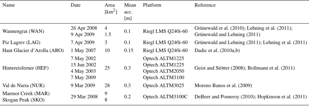
Table 1. Data sets. “Date” is the date of the winter survey, “Area” the area of the data set, “Mean acc.” the mean accuracy in vertical direction as quoted in the reference column and “Platform” the measurement plaform.
Name Date Area Mean Platform Reference
[km2] acc.
[m]
Wannengrat (WAN) 26 Apr 2008 4 0.1 Riegl LMS Q240i-60 Gr¨unewald et al. (2010); Lehning et al. (2011);
9 Apr 2009 1.5 Gr¨unewald and Lehning (2011)
Piz Lagrev (LAG) 7 Apr 2009 3 0.1 Riegl LMS Q240i-60 Gr¨unewald and Lehning (2011); Lehning et al. (2011)
Haut Glacier d’Arolla (ARO) 1 May 2007 10 0.15 Riegl LMS Q240i-60 Dadic et al. (2010a,b)
Hintereisferner (HEF)
7 May 2002
25 0.3
Optech ALTM1225
Geist and St¨otter (2008); Bollmann et al. (2011)
15 Jun 2002 Optech ALTM1225
4 May 2003 Optech ALTM2050
7 May 2009 Optech ALTM3100
Val de Nuria (NUR) 9 Mar 2009 28 0.3 Optech ALTM3025 Moreno Banos et al. (2009)
Marmot Creek (MAR)
29 Mar 2008 9 0.2 Optech ALTM3100C DeBeer and Pomeroy (2010); Hopkinson et al. (2011)
Skogan Peak (SKO) 8
the system to be tilted in the direction of the target (im-proved incident angel) results in a higher accuracy. Compar-ing helicopter-based snow depth maps with terrestrial laser scanning and tachymeter surveys, Gr¨unewald et al. (2010) found that the error of the ALS data was below 10 cm. The typical area covered by ALS data sets obtained for this study is between 1 and 30 km2and they all have a spatial resolu-tion close to one metre. Accuracy estimaresolu-tions and references to the data analyzed in this study are given in Table 1.
2.2 Site description
We assembled a large data set consisting of seven investi-gation areas located in six different regions, including the Swiss and the Austrian Alps, the Spanish Pyrenees, and the Canadian Rocky Mountains. Two catchments are dominated by glaciers whereas the remaining areas are free of ice. The borders of the investigation areas analysed in this study have been defined manually. This study focuses on the snow depth distribution of alpine areas. Therefore, effects of vegetation, such as interception of snow by trees, were not considered and all parts of the investigation areas which are covered by significant vegetation were masked from the data. Further-more, it has been shown that ALS snow depth measurements are more accurate over alpine areas than adjacent forest cov-ered areas (Hopkinson et al., 2012). In the following, we give a brief overview of the study sites. For more details, the reader may refer to Table 1, Figs. 1 to 3 and to the references given in the text.
2.2.1 Wannengrat, CH
The Wannengrat (WAN) area (Fig. 1a) is a small alpine catchment that is located in the eastern part of the Swiss Alps. The site has been an intensive investigation area for snow studies in recent years (Gr¨unewald et al., 2010; Gr¨unewald and Lehning, 2011; Mott et al., 2010, 2011, 2013; Schirmer
et al., 2011; Schirmer and Lehning, 2011; Wirz et al., 2011; Egli et al., 2012). Most of the area is above the local tree line and no tall vegetation is present. Elevations range from 1940 to 2650 m a.s.l. and the lower part is typically char-acterised by gentle slopes whereas the summit region is formed by talus and steep rock faces. Storms which domi-nate the snow accumulation in the area usually come from the north-west (Mott et al., 2010; Schirmer et al., 2011). Two helicopter-based (Vallet and Skaloud, 2005; Skaloud et al., 2006; Vallet, 2011) winter ALS data sets were obtained in the area on 26 April 2008 and 9 April 2009, which repre-sent the maximum snow accumulation in the area for the two years. The area of the second flight covers 5 km2, whereas the first flight only covers a small part of the domain (1.5 km2, see Gr¨unewald et al., 2010; Gr¨unewald and Lehning, 2011).
2.2.2 Piz Lagrev, CH
The Piz Lagrev (LAG) study area (Fig. 1b) includes the south face of the Piz Lagrev, which is part of the mountain range defining the northern rim of the Engadin valley in the south-east of the Swiss Alps. The site is above the local tree line, and elevations range from 1800 to 3080 m. The Piz Lagrev is characterised by steep talus slopes which are surrounded by steep rock faces. Two pronounced, sheltered bowls dominate the upper part of the area (Gr¨unewald and Lehning, 2011). ALS measurements were obtained on 7 April 2009 using the same technology as for the Wannengrat, and cover an area of about 5 km2. Analysis of a nearby weather station indicates that the prevailing wind direction is south-west.
2.2.3 Haut Glacier d’Arolla, CH
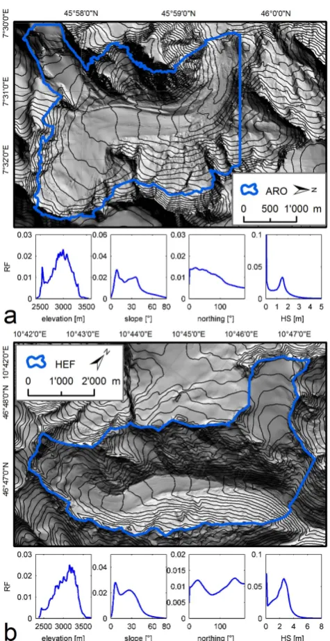
Fig. 1. Hillshade map of (a) the Wannengrat (WAN) and (b) the Piz Lagrev (LAG) study areas. The contour lines have an equidis-tance of 50 m. The right panels show histograms for elevation, slope, northing and the area-wide absolute snow depth obtained from ALS. Data source basemap: (a, b) DOM-AV©2012 swisstopo (5704 000 000).
by the 4.4 km2Haut Glacier d’Arolla and by several smaller cirque glaciers. About 50 % of the area is glaciated and the rest of the domain is characterised by steep slopes and rock faces. Helicopter-based Lidar measurements of the area were obtained in November 2006 and May 2007 (Dadic et al., 2010a,b). The resulting snow depth map represents the time of the maximum snow accumulation for at least the high re-gions of the catchment. According to Dadic et al. (2010a),
Fig. 2. Hillshade map of (a) Haut Glacier d’Arolla (ARO) and (b) the Hintereisferner (HEF) study areas. The contour lines have an equidistance of 50 m. The right panels show histograms for el-evation, slope, northing and the area-wide absolute snow depth obtained from ALS (for HEF: Mai 2002). Data source basemap: (a) DOM-AV©2012 swisstopo (5704 000 000); (b) Land Tirol – http://data.tirol.gv.at.
[image:5.595.50.284.61.528.2]zone, whereas the overestimation in the ablation zone may be countered by the previously mentioned surface melt. An analysis of weather stations in the surrounding area showed that wind directions are variable, but that the synoptic main flow is from the southwest. This is also confirmed by tempo-rary measurements in the catchment (Dadic et al., 2010a,b).
2.2.4 Hintereisferner, AT
The investigation area Hintereisferner (HEF) is situated in the upper Rofen valley, which is part of the ¨Otztal Alps at the Austrian–Italian border (Fig. 2b). The catchment, as de-fined for this study, covers an area of 25 km2 and is char-acterised by glaciers, steep slopes and rock faces. Eleva-tions range from 2300 to 3740 m a.s.l. and the largest glaciers are the valley glacier Hintereisferner (2002:∼6.5 km2) and
the Kesselwandferner (2002:∼3.8 km2). On the local scale, wind directions are very variable, but the main direction is northwest. In this study, we analyze data obtained in three measurement campaigns in the beginning of May 2002, 2003 and 2009, and one data set acquired in June 2002 (Geist and St¨otter, 2008, Table 1). The first three flights were near the end of the seasonal snow accumulation in the area, whereas snowmelt clearly had an effect on the lower parts of the catchment in June 2002. To calculate snow depth, each of the winter DSMs was subtracted from a summer DEM ob-tained in the previous autumn of the respective year. As for ARO, glacier dynamics were neglected in the calcula-tions. More details on the investigation area and the ALS campaigns can be found in Geist and St¨otter (2008) and Bollmann et al. (2011).
2.2.5 Vall de N ´uria, ES
Vall de N´uria (NUR) (Fig. 3a) is located at the main di-vide in the Eastern part of the Spanish Pyrenees. An ALS campaign covering an area of 38 km2 was performed on 9 March 2009, which is near the time of the peak of the sea-sonal accumulation for the area (Moreno Banos et al., 2009). After masking significant vegetation and human infrastruc-ture 28 km2 of the area remained. Elevations range from 2000 to 2900 m a.s.l. and the mean slope is 28◦. The area is characterised by a mixture of gentle slopes and some steeper, rocky areas in the summit region. The most frequent synoptic wind direction in the area is from the northwest, even though a large variability of the wind direction is present on the local scale.
2.2.6 Marmot Creek, CA
[image:6.595.309.546.63.523.2]Marmot Creek Research Basin in the Kananaskis Valley, Alberta is located within the Front Range of the Canadian Rocky Mountains. For our analysis we selected two small do-mains (Fig. 3b). The investigation area named Marmot Creek (MAR) in this study is the alpine zone surrounding Mount Allan and includes the Marmot Creek basin in the East. The
Fig. 3. Hillshade map of (a) the Val de N´uria (NUR) and (b) Mar-mot Creek Research Basin area with the study areas MarMar-mot Creek (MAR) and Skogan Peak (SKO). The contour lines have an equidis-tance of 50 m. The panels below show histograms for elevation, slope, northing and the area-wide absolute snow depth obtained from ALS.
elevation range is 1660 to 2660 m a.s.l. SKO is characterised by very rough topography with steep slopes and rock faces (average slope 40◦). Only small areas have gentle terrain. Airborne Lidar surveys of the snow cover were obtained at 29 March 2008. The time of the flight did not coincide with the maximum of the seasonal snow accumulation in the area, which was reached in mid-May (DeBeer and Pomeroy, 2010; Hopkinson et al., 2012). The snow cover in the complete area is strongly affected by winds, which mainly come from the northwest to Fisera Ridge in MAR but generally come from the southwest (MacDonald et al., 2010). Further information on the area and the climatic conditions can be found in De-Beer and Pomeroy (2010), MacDonald et al. (2010), Marsh et al. (2012) and Pomeroy et al. (2012).
2.3 Aggregation of sub-areas
The aim of this study is to explain the spatial variability of snow depth on the catchment scale. With high-resolution snow depth measurements at hand, a statistical assessment considering snow depth and topography at the highest pos-sible resolution is not meaningful. The difficulty becomes obvious if one thinks about cornices or other drift features. Maximum snow depth in a cornice is not the result of to-pographic features (e.g. slope) directly at this point but is shaped by the upwind topography interacting with the wind. Therefore, a systematic correlation between snow depth and terrain parameters will not be found at very small scales. Re-gression models of snow depth of the different investigation areas (not shown) confirmed that and showed that at the high-est resolution (metre scale without aggregation), only 2 to 37 % of the variability could be explained by the terrain. Because of the large spatial variability at scales of metres (Shook and Gray, 1996; Watson et al., 2006), we define sub-areas in order to smooth this small-scale variability. We ag-gregated the data to spatially continuous subareas with length scales of some hundreds of metres.
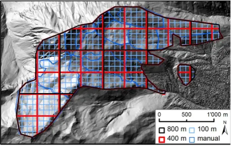
[image:7.595.310.546.63.212.2]Two different methods for the aggregation are applied. The first is the same as performed by Lehning et al. (2011), who manually defined sub-areas from a subjective impression of the terrain (Fig. 4). The length scale of these subareas was ap-proximately 500 m. Such an aggregation follows the concept of hydrological response units (HRU), which has success-fully been applied for semi-distributed hydrological mod-els (Kite and Kouwen, 1992; Rinaldo et al., 2006; Pomeroy et al., 2007) and is consistent with the concept of stratified snow sampling (Steppuhn and Dyck, 1974) where landscape units were defined to minimise within-unit variance of SWE and maximise difference in SWE between units. The facets applied by Daly et al. (1994) for the calculation of precip-itation gradients or to the concept of snow accumulation units outlined by Hopkinson et al. (2012) are also similar ap-proaches. The second method is a simple automatic approach which divides the domain into quadratic subareas. This ap-proach is very similar to a simple resample of the data to
Fig. 4. Aggregation of sub-aras for the Wannengrat area by the man-ual and the automatic method (grids of different cell size).
larger cell sizes. We have tested different grid sizes ranging from 100 to 800 m. An example which illustrates the aggre-gation is shown in Fig. 4. The criteria which were applied to select the cell size appropriate for the study are: (i) the small scale variability should be smoothed out to an extent that the remaining variability can be reasonably explained by the topographic parameters, and (ii) the number of sub-areas must be large enough to be able to fit robust regression mod-els (N'30). In order to avoid small clusters which do not represent a significant footprint of the catchment, very small sub-areas (<10 000 m2) were automatically excluded from the aggregated data. The approach is similar to the concept of representative elementary area (Wood et al., 1988; Bl¨oschl et al., 1995), which aims to identify ideal scales for hydrolog-ical modelling applications.
As the second method is a straightforward and fully auto-mated approach, it is possible to compose multiple statisti-cal models by randomly shifting the origin of the grid. This approach helps to identify the range of model performance and if a selected grid results in a representative model. The impact of random effects, which might be caused by a sin-gle grid or by subjective classification of the sub-areas, can therefore be assessed.
2.4 Statistical models
between windward and leeward slopes (Pomeroy and Brun, 2001). In order to be able to combine data sets from differ-ent areas, elevation was changed to relative elevation (dE), which is the difference between the absolute and the mini-mum elevation of the area. This mapping respects the fact that all data sets are from the alpine zone at or above tree line but that this corresponds to different absolute elevation in the different areas. The slope (SL) represents gravitational pro-cesses such as sloughing and avalanching, which can have a significant effect on the snow distribution (Bl¨oschl and Kirnbauer, 1992; Gruber, 2007; Sovilla et al., 2010; Bern-hardt and Schulz, 2010). In combination with northing (NO), the slope also describes the amount of solar energy which is available for the ablation and settling of snow. NO is also important for the deposition and redistribution of snow by wind (Seyfried and Wilcox, 1995; Lehning et al., 2008), as more snow is usually accumulated in the leeward sides of slopes and mountains. An additional parameter, which rep-resents the effect of the wind, is the mean sheltering index SX (Winstral et al., 2002), which has been calculated for the direction of the main flow (see site descriptions) and for a maximum distance of 100 m. Several studies showed that SX is a good measure for sheltering and exposure of the lo-cal terrain, which gives a simple but reasonable representa-tion of the local flow field and therefore of the redistriburepresenta-tion of snow by wind (e.g. Winstral and Marks, 2002; Winstral et al., 2002; Anderton et al., 2004; Erickson et al., 2005; Molotch et al., 2005; Litaor et al., 2008; Schirmer et al., 2011). Finally, different measures for the surface roughness are applied. The standard deviation of the elevation (σ (E)) and slope (σ(SL)) represent classical morphometric rough-ness measures (Evans, 1972; Speight, 1974; Shepard et al., 2001). The surface roughness strongly affects the redistribu-tion of snow by wind and gravitaredistribu-tional processes (Jost et al., 2007), and can be seen as the capability of the surface to trap snow. As suggested by Lehning et al. (2011), we also tested the fractal dimensionDand the ordinal interceptγ of the semi-variogram, which have been identified as good mea-sures for the surface roughness (Goodchild and Mark, 1987; Power and Tullis, 1991; Klinkenberg, 1992; Klinkenberg and Goodchild, 1992; Xu et al., 1993; Sun et al., 2006; Taud and Parrot, 2006).
For each of the aggregated data sets, we separately calcu-lated all possible two- and three-parameter regression models and selected the most significant models (pvalue<0.001). Further selection criteria are the explanatory power (R2) of the model and – if theR2was similar – the number of pa-rameters included in the model. For data sets with a two-parameter model, which had a similar performance as the best three-parameter-model, the two-parameter-model was selected. To account for possible interactions of the param-eters included in the models, factor combinations (multipli-cation of parameters) have been tested and included where appropriate. The preconditions of linear regression (nor-mal distribution and constant variance of residuals) were
examined by analyzing the Quantil–Quantil plots and the Tukey–Anscombe plots of the model residuals (not shown). Additionally, the physical meaningfulness of the models (e.g. sign of the coefficients) has been examined, and mod-els have not been selected if the sign of the coefficient was counter-intuitive. As mentioned before, the automatic aggre-gation to quadratic sub-areas allows the calculation of multi-ple random grids. This in turn can be used to analyse whether the best models are consistent (same explanatory variables) and show a small standard deviation of the coefficients when calculated for different grid realizations. Note that the frac-tal parametersDandγ could not be included in the multi-ple model runs, as their computation is computationally very demanding. D and γ were therefore only applied for the models with manually defined sub-areas and for few selected quadratic models.
To assess the transferability of the results, we also built a “global” model by combining all data sets. In addition, sub-sets of the data were combined based on their morphologi-cal characteristics. The two morphologimorphologi-cal models discussed here are “Glacier”, which includes the two sites which are currently glaciated, and “No glacier”, which combines all re-maining, non-glaciated data sets from alpine terrain.
The multiple-year data sets for HEF and WAN allow a val-idation in order to investigate the inter-annual consistency of the models. For HEF, models calculated from data sets con-taining three of the snow depth surveys in the area are vali-dated with the remaining years. We repeated this procedure for each combination. Scatter plots and the coefficients of determination (R2det) are used to assess the performance of the validation. As the extent of the 2008 data set for WAN is very small it could not be used to compose an own re-gression model. Nonetheless it could be used to validate the model obtained from the 2009 data set.
3 Results and discussion
3.1 Aggregation of sub-areas
Table 2. Best two- to three-parameter model for each single investigation area, where dHS and dEare in metres and SL and NO in degree. Column 3 to 5 show theR2, the adjustedR2(R2Adj) and the number of sub-areas for each model. For HEF all data (four points of time) were combined to one single model.
Area Model R2 RAdj2 N
WAN dHS = 0.00153·dE −0.0240·SL −0.0043·NO +0.60 0.76 0.73 35
LAG dHS = 0.00202·dE −0.0574·SL +1.39 0.91 0.90 29
NUR dHS = −0.0005·NO +0.56·SX +0.1715·σ(SL) −0.0012·NO·σ(SL) −0.49 0.50 0.49 222 MAR dHS = −0.0115·SL −0.0025·NO +0.77·SX −0.0049·NO·SX +0.61 0.30 0.27 66
SKO dHS = −0.0363·SL −0.0074·NO +0.59·γ +1.84 0.41 0.38 66
ARO dHS = 0.00246·dE −0.0009·SL −0.0032·NO −4.054×10⁻⁵dE·SL −0.26 0.53 0.50 82
HEF∗ dHS = 0.00182·dE −0.0385·SL −0.0024·NO +0.05 0.51 0.50 720
∗includes HEF(05-2002), HEF(06-2002), HEF(05-2003), HEF(05-2009).
remains large enough to calculate robust statistical models. For the other investigation areas, similar results (not shown) were obtained. Cell sizes between 200 and 500 m showed to perform best. This is consistent with the length scale of >100 m found by Shook and Gray (1996) for minimal au-tocorrelation in snow depth data. We therefore decided to apply a grid size of 400 m to all areas. Choosing a 200 m grid instead of the 400 m would result in very similar mod-els but with lower performance: while the model parameters remain the same, the modelledR2would be reduced by 0.01 to 0.14 for the different data sets. For example for WAN R2would decrease from 73 to 59 % (Fig. 5b). Moreover, a 400 m grid is a similar level of aggregation as for the man-ually defined sub-areas. A comparison of models, calculated with sub-areas identified by the manual and the automatic (400 m) approach, showed that the results are very similar in terms of the best parameters selected for the final models, and in terms of model performance. As it is an objective and fully automatic method, we only show results from the automatic procedure in the following.
3.2 Statistical models
The model assumptions for linear regressions (see above) were fulfilled satisfactorily for all data. Nevertheless, small deviations from the normal distribution of residuals for very large positive and negative residuals have to be reported for ARO, HEF and SKO. Logarithmic transformation of the vari-ables has been tested. As this did not yield improvements, the original, non-transformed variables were used.
3.2.1 Single catchment models
[image:9.595.310.546.238.453.2]Table 2 summarises the best models for each of the sin-gle investigation areas. The table indicates that similar pa-rameter combinations dominate most areas. Such, dE, NO and SL are included in almost all models. SX is included for NUR and for MAR. A roughness index is only present in the model for NUR (σ(SL)) and SKO (γ). Nevertheless substituting γ by, for example, (σ(SL)) would result in a model with a similar performance. For some areas, different
Fig. 5. Relationship between the level of aggregation (cell size) and snow depth variability expressed by (a) the standard deviation σ(HS), and (b) model performance (R2) for the Wannengrat area (model with dE, SL, NO). The black circles indicate the mean of 50 random model runs. TheR2of each run is induced by a small black dot. The red dots show the average number of sub-areas (N) at each aggregation level.
parameter combinations than the ones presented have only a slightly lower performance (not shown). Factor combination significantly improved the model for NUR, MAR and ARO. Adding an additional parameter would further improve the models for some of the areas (NUR, MAR, SKO). In order to keep the models as simple as possible and to avoid an over-parameterization of the small areas, we do not include such additional variables.
(2 cm (◦SL)−1) and a decrease of dHS toward southerly
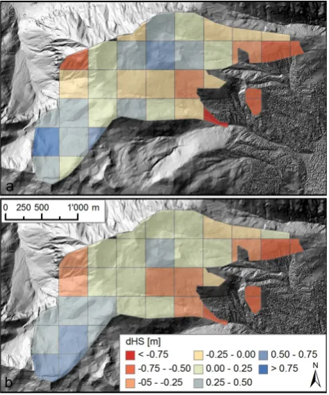
as-pects (4 cm (10◦NO)−1). Figure 6 compares a dHS map
resulting from the model with measured dHS, aggregated to the model resolution. The upper image shows the snow depth distribution as aggregated from the ALS measure-ments, while the lower image presents the snow cover as cal-culated with the model. The figure illustrates that the statis-tical approach seems suitable to characterise the general spa-tial patterns of the snow depth distribution. Deviations occur especially in regions of extreme dHS, for example, in single cells in the northwest, the southeast or the southwest. This indicates that the model does not properly capture the ex-tremes of the distribution. Nevertheless, the deviations are only small.
Returning to Table 2 and focussing on the different ar-eas, it appears that both the parameters and the model co-efficients are varying between the data sets. It is also obvi-ous that the performance of the models (R2) is quite differ-ent. While the model for LAG can explain more than 90 % of the snow depth variability, only 30 % could be explained for MAR and 41 % for SKO. For most areas, theR2is be-tween 50 and 70 % which is a very good score in compari-son to published results obtained at similar scales. The large range in the model performance might be attributed to the topographic diversity within the single catchments. Smaller, less heterogeneous catchments, such as LAG or WAN per-form much better than the very large (HEF, ARO, NUR) or very complex (MAR, SKO) areas. Reasons for the relatively lowR2 for MAR and SKO can be found in the character-istics of the data sets, where the topography in the summit region of the two areas is dominated by extremely steep rock faces (Fig. 3b), which are exposed to wind and avalanches. In the period before the snow depth data had been acquired, several heavy storms occurred in the area. The heavy winds eroded and sublimated much of the snow cover in the sum-mit region and, as a result, the major portion of the sumsum-mit region was nearly free of snow. This is a common character-istic of alpine snow in the relatively windy Canadian Rockies (MacDonald et al., 2010). A further possible reason for the lower performance of some of the models could be the ac-curacy of some parts of the ALS data. As mentioned before, it must be expected that biases are larger in steep and rough terrain, especially for the data obtained from airplanes. Such terrain-based errors will also influence the models on resolu-tions as presented here and must be considered when inter-preting results from such areas, especially when slope serves as an explanatory variable.
[image:10.595.310.547.63.348.2]In general, the results confirm that topography dominates the snow depth distribution at that scale. The deviations be-tween the models indicate that the influences on the snow depth distribution are variable in the different areas. For ex-ample, the magnitude of the elevation gradient is between 6 and 25 cm/100 m, and the coefficient for slope varies by a factor of four (ARO not included because of factor combina-tions). For NUR and MAR, the elevation gradient dEseems
Fig. 6. Comparison of dHS for the Wannengrat in April 2009, ag-gregated to (a) a 400 m grid form ALS-measurements, and (b) mod-elled with a regression model with dE, SL and NO.
not to be relevant at all. Instead, the sheltering effect of the terrain (SX) is more important.
The representativeness of the results obtained from the selected grid (Table 2, Fig. 4) was assessed by calculating multiple model runs, for which the origins of the grid were shifted randomly. Results are summarised in Table 3. Fifty runs were performed for the best model, as identified in Ta-ble 2 (but without factor combinations), for each investiga-tion area. The table shows the sample space (25 to 75 % quantiles) for all model parameters and for the model per-formance. The last column indicates theR2of the model run that is based on the same grid as the models presented in Table 2.
Generally the table indicates relatively small interquan-tile ranges for most models and parameters. For example for WAN (first line) the difference between the upper and lower quantile and the median ofαi is only 6 to 10 % of the me-dian. Similar ranges are characteristic for most parameters in the other data sets. Onlyα1 andα3 for SKO andα3 for
Table 4. Best models,R2,R2Adjand number of subareas (N) for different combinations of the investigation areas.
Area Model R2 R2
Adj N
Alla dHS = 0.00079·dE −0.0145·SL −0.0028·NO +0.28 0.23 0.22 682
No Glacierb dHS = −0.0133·SL −0.00528·NO +0.0454·σ(SL) +0.53 0.30 0.29 423 Glacierc dHS = 0.00021·dE −0.0686·SL +5.329×10⁻⁵dE·SL +0.79 0.48 0.48 802
Included data sets:
aWAN, LAG, NUR, MAR, SKO, ARO, HEF(05-2001);bWAN, LAG, NUR, MAR, SKO;cARO, HEF(05-2002), HEF(06-2002), HEF(05-2003), HEF(05-2009).
the single runs is only moderate. Taken as a whole, Table 3 shows that most of the models represent the total average well. Moreover, we can conclude that the absolute position of the subareas only has a minor effect on the models. The spatial averaging procedure appears to result in relatively sta-ble statistical relations, at least at the scale of the 400 m grid.
3.2.2 Combined models
For practical applications on a large scale, it would be very beneficial if it were possible to find a “global” model, which would be able to predict a large portion of the spatial vari-ability for all data sets. We therefore combined all data to one large data set and built a new model, following the same pro-cedure described above. However, the resulting model (Ta-ble 4), which selected dEand SL as explanatory variables, was only able to explain 23 % of the total snow depth vari-ability of the aggregated data. Additional model parameters or factor combinations could not significantly improve the model. A model that only includes data from the alpine areas, which are presently not glaciated, is capable of explaining 30 % of the variability. This is clearly worse than the mod-els for most of the single data sets (Table 2). It appears that as suggested by Pomeroy and Gray (1995), the interaction between topography and snow depth is not the same at dif-ferent sites, and that a statistical relationship, developed for one area, cannot directly be transferred to a different site. In contrast, the “glacier” model features a similar performance to the models for the single glaciers (ARO and HEF). This could indicate that similar characteristics are important for the snow cover on glaciated catchments or that the sample size is too small to show substantial variability in glaciated sites. However, since the model consists of the same data as the HEF model presented in Table 2, only supplemented by the comparably small ARO data, the ARO data will only have a minor effect on the model and itsR2value.
Finally, when combining data sets from different sources, one needs to be aware of possible differences in the platforms and sensors applied for the data acquisition. Sensors of dif-ferent manufacturers can be very diverse in their design, op-erational envelope and laser pulse specifications which might result in different levels of performance and error propaga-tion. Nevertheless, the influence on statistical relationships should be marginal.
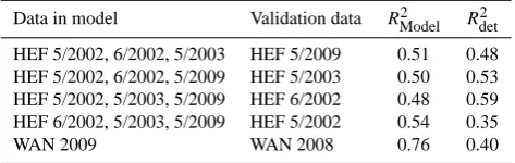
Table 5. Inter-annual consistency for HEF and WAN. The first col-umn lists the data which were used to fit the model (model param-eters dE, SL, NO). The second column shows the data set used for the validation.RModel2 is theR2of the model, andR2detthe coeffi-cient of determination.
Data in model Validation data RModel2 Rdet2
HEF 5/2002, 6/2002, 5/2003 HEF 5/2009 0.51 0.48 HEF 5/2002, 6/2002, 5/2009 HEF 5/2003 0.50 0.53 HEF 5/2002, 5/2003, 5/2009 HEF 6/2002 0.48 0.59 HEF 6/2002, 5/2003, 5/2009 HEF 5/2002 0.54 0.35
WAN 2009 WAN 2008 0.76 0.40
3.2.3 Inter-annual consistency
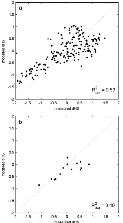
Results of the analysis of the inter-annual consistency, as de-scribed in Sect. 3.2.1, are shown in Table 5. Figure 7 illus-trates the scatter plots for the validation, as shown in lines two (a) and five (b) of Table 5. The table emphasizes that the Rdet2 values are around 50 %, which is similar to theR2 val-ues of the full models. Only WAN and the fourth HEF model have a lowerR2det. Nevertheless, Fig. 7b shows that for the WAN data the model is appropriate for both years for most sub-areas.
[image:12.595.311.548.253.328.2]Fig. 7. Measured vs. modelled (parameters: dE, SL and NO) dHS for (a) HEF and (b) WAN. For HEF, the snow depth data obtained in May 2003 are validated in a model calculated with the data from May 2002, June 2002 and May 2009. For WAN, the model from 2009 is validated with data from 2008.
who concluded that few major storms shape the snow depth distribution at the end of the winter, supports that hypothesis.
4 Conclusions
In this paper, we have applied linear multiple-regression modelling of snow depth distributions with topographic pa-rameters for several small and medium size catchments in different mountain regions of the world. We showed that sta-tistical modelling is capable of explaining large parts of the spatial distribution of snow depth on the catchment scale. This is only achieved if the data is aggregated to length scales of some hundreds of metres, in order to smooth out the very large heterogeneity caused by drifting snow at small scales. After arbitrary clustering of the data to quadratic cells with a grid size of 400 m, 30 to 91 % of the variability could be
explained by including only three explanatory parameters. For the first time, a systematic investigation of the explana-tory power as a function of scale has been made. The param-eters which are most frequent in the models are the eleva-tion gradient (dE), the slope (SL), a substitute for the aspect (NO), and a wind-sheltering index (SX). These results are typically better than those obtained by other studies because of the systematic aggregation. It is important to notice that owing to the high resolution of the original data applied in our study, the full small-scale variability of the snow cover is captured. This is not the case for most earlier studies, which had to rely on a limited number of point observations, such as snow stakes or SNOTEL sites. This means that not only is it likely that the full variability is not represented in these data sets, but also that there is a potential bias in the data, e.g. if only flatter portions of a catchment are sampled (Wirz et al., 2011).
Studies which compare data from different regions are also rare. Our analysis showed that there are clear differences be-tween the models for the specific regions, but that a global model still explains a significant fraction of the variability (23 or 30 % without glaciers). This indicates that the relation-ship between snow and topography is less universal than hy-pothesized by Lehning et al. (2011) and the application of a “global” model is limited. On the contrary, it could be shown that statistical models, developed for one year, can be well applied to other years, at least for the points of time of the maximum seasonal accumulation. This is an important find-ing for applications in hydrology or glaciology. A method, as presented here, can serve as a straightforward approach to characterise the spatial distribution of the snow cover. Ap-plications from year to year should be applied with caution in some areas which have been reported to show high inter-annual changes in wind regimes that transport blowing snow. We expect that more area-wide snow depth data sets will become available in the coming years. It might soon be pos-sible to cover a larger spectrum of mountain regions for all over the world.
It will be interesting to see if the main topographic pa-rameters that provided some explanation of snow depth dis-tributions here for a limited section of climatic and physio-graphic environments are also important in other environ-ments. Combining statistical with parametric or physically based methods might also yield more robust, yet still simple, models of snow accumulation. Another question which needs to be addressed is if such statistical relations are also valid for different points of time during the snow season, and how the statistical relationships change with time. This would require area-wide snow depth data for a larger area from different points of time during a season.
Acknowledgements. We want to acknowledge all our colleagues
including R. Mott, M. Schirmer, E. Trujillo, P. Oller, C. DeBeer, C. Ellis, M. MacDonald, M. Solohub, T. Collins, J. Churchill and many more, who contributed to field work, data processing or with feedback and good ideas. For his efforts with language editing we thank M. von Pokorny. The ALS campaigns were supported and partly founded by the Amt f¨ur Wald Graub¨unden, the IP3 Cold Regions Hydrology Network, the Government of Alberta – (En-vironment and Sustainable Resources Development), C-CLEAR (Canadian Consortium for LiDAR Environmental Applications Research) and the Geological Survey of Canada. Parts of the work have also been founded by the Swiss National Foundation. We finally thank the editor M. Weiler, S. Pohl and two anonymous reviewers for their constructive comments and corrections.
Edited by: M. Weiler
References
Anderton, S. P., White, S. M., and Alvera, B.: Evaluation of spatial variability in snow water equivalent for a high mountain catch-ment, Hydrol. Process., 18, 435–453, doi:10.1002/Hyp.1319, 2004.
Balk, B. and Elder, K.: Combining binary decision tree and geostatistical methods to estimate snow distribution in a mountain watershed, Water Resour. Res., 36, 13–26, doi:10.1029/1999wr900251, 2000.
Baltsavias, E.: Airborne laser scanning: basic relations and formu-las, J. Photogramm. Remote Sens., 54, 199–214, 1999.
Bavay, M., Lehning, M., Jonas, T., and L¨owe, H.: Simulations of fu-ture snow cover and discharge in Alpine headwater catchments, Hydrol. Process., 23, 95–108, doi:10.1002/hyp.7195, 2009. Bavay, M., Gr¨unewald, T., and Lehning, M.: Response of snow
cover and runoff to climate change in high Alpine catch-ments of Eastern Switzerland, Adv. Water Resour., 55, 4–16, doi:10.1016/j.advwatres.2012.12.009, 2013.
Beniston, M., Keller, F., and Goyette, S.: Snow pack in the Swiss Alps under changing climatic conditions: an empirical approach for climate impacts studies, Theor. Appl. Climatol., 74, 19–31, doi:10.1007/s00704-002-0709-1, 2003.
Bernhardt, M. and Schulz, K.: SnowSlide: A simple routine for cal-culating gravitational snow transport, Geophys. Res. Lett., 37, L11502, doi:10.1029/2010gl043086, 2010.
Bernhardt, M., Z¨angl, G., Liston, G. E., Strasser, U., and Mauser, W.: Using wind fields from a high-resolution atmo-spheric model for simulating snow dynamics in mountainous terrain, Hydrol. Process., 23, 1064–1075, doi:10.1002/hyp.7208, 2009.
Bl¨oschl, G. and Kirnbauer, R.: An analysis of snow cover patterns in a small alpine catchment, Hydrol. Process., 6, 99–109, 1992. Bl¨oschl, G., Grayson, R. B., and Silvaplana, M.: On the
repre-sentative elementary area (REA) concept and its utility for dis-tributed rainfall-runoff modeling, Hydrol. Process., 9, 313–330, doi:10.1002/hyp.3360090307, 1995.
Bollmann, E., Sailer, R., Briese, C., Stotter, J., and Fritzmann, P.: Potential of airborne laser scanning for geomorphologic fea-ture and process detection and quantifications in high alpine mountains, Z. Geomorphol., 55, 83–104, doi:10.1127/0372-8854/2011/0055s2-0047, 2011.
Chang, K. T. and Li, Z. X.: Modelling snow accumulation with a geographic information system, Int. J. Geogr. Inf. Sci., 14, 693– 707, 2000.
Choularton, T. W., and Perry, S. J.: A model of the oro-graphic enhancement of snowfall by the seeder-feeder mechanism, Q. J. Roy. Meteorol. Soc., 112, 335–345, doi:10.1002/qj.49711247204, 1986.
Clark, M. P., Hendrikx, J., Slater, A. G., Kavetski, D., Anderson, B., Cullen, N. J., Kerr, T., Hreinsson, E. O., and Woods, R. A.: Rep-resenting spatial variability of snow water equivalent in hydro-logic and land-surface models: a review, Water Resour. Res., 47, W07539, doi:10.1029/2011wr010745, 2011.
Cline, D., Elder, K., and Bales, R.: Scale effects in a dis-tributed snow water equivalence and snowmelt model for mountain basins, Hydrol. Process., 12, 1527–1536, doi:10.1002/(sici)1099-1085(199808/09)12:10/11<1527::aid-hyp678>3.0.co;2-e, 1998.
Dadic, R., Corripio, J. G., and Burlando, P.: Mass-balance estimates for Haut Glacier d’Arolla, Switzerland, from 2000 to 2006 using DEMs and distributed mass-balance modeling, Ann. Glaciol., 49, 22–26, 2008.
Dadic, R., Mott, R., Lehning, M., and Burlando, P.: Wind influence on snow depth distribution and accumulation over glaciers, J. Geophys. Res.-Earth, 115, 8, doi:10.1029/2009JF001261, 2010a. Dadic, R., Mott, R., Lehning, M., and Burlando, P.: Parameteriza-tion for wind-induced preferential deposiParameteriza-tion of snow, Hydrol. Process., 24, 1994–2006, doi:10.1002/hyp.7776, 2010b. Daly, C., Neilson, R. P., and Phillips, D. L.: A
statistical-topographic model for mapping climatological precipitation over mountainous terrain, J. Appl. Meteorol., 33, 140–158, doi:10.1175/1520-0450(1994)033<0140:astmfm>2.0.co;2, 1994.
DeBeer, C. M. and Pomeroy, J. W.: Simulation of the snowmelt runoff contributing area in a small alpine basin, Hydrol. Earth Syst. Sci., 14, 1205–1219, doi:10.5194/hess-14-1205-2010, 2010.
Deems, J. S., Fassnacht, S. R., and Elder, K. J.: Fractal distribution of snow depth from lidar data, J. Hydrometeorol., 7, 285–297, 2006.
Deems, J. S., Fassnacht, S. R., and Elder, K. J.: Interan-nual consistency in fractal snow depth patterns at two Colorado mountain sites, J. Hydrometeorol., 9, 977–988, doi:10.1175/2008jhm901.1, 2008.
Egli, L., Jonas, T., Gr¨unewald, T., Schirmer, M., and Burlando, P.: Dynamics of snow ablation in a small Alpine catchment observed by repeated terrestrial laser scans, Hydrol. Process., 26, 1574– 1585, doi:10.1002/hyp.8244, 2012.
Elder, K., Dozier, J., and Michaelsen, J.: Snow accumulation and distribution in an Alpine watershed, Water Resour. Res., 27, 1541–1552, doi:10.1029/91wr00506, 1991.
Elder, K., Rosenthal, W., and Davis, R. E.: Estimating the spatial distribution of snow water equivalence in a montane watershed, Hydrol. Process., 12, 1793–1808, 1998.
Erxleben, J., Elder, K., and Davis, R.: Comparison of spatial interpolation methods for estimating snow distribution in the Colorado Rocky Mountains, Hydrol. Process., 16, 3627–3649, doi:10.1002/Hyp.1239, 2002.
Essery, R., Martin, E., Douville, H., Fernandez, A., and Brun, E.: A comparison of four snow models using obser-vations from an alpine site, Clim. Dynam., 15, 583–593, doi:10.1007/s003820050302, 1999.
Evans, I. S.: General geomorphometry, derivatives of altitude, and descriptive statistics, in: Spatial Analysis in Geomorphology, edited by: Chorley, R., Harper & Row, London, 17–90, 1972. Fang, X. and Pomeroy, J. W.: Modelling blowing snow
redistri-bution to prairie wetlands, Hydrol. Process., 23, 2557–2569, doi:10.1002/hyp.7348, 2009.
Frei, C. and Sch¨ar, C.: A precipitation climatology of the Alps from high-resolution rain-gauge observations, Int. J. Climatol., 18, 873–900, 1998.
Geist, T. and St¨otter, J.: Documentation of glacier surface elevation change with multi-temporal airborne laser scanner data – case study: Hintereisferner and Kesselwandferner, Tyrol, Austria, Z. Gletscherk. Glazialgeol., 41, 77–106, 2008.
Geist, T., H¨ofle, B., Rutzinger, M., and St¨otter, J.: Laser Scanning – a paradigm change in topographic data acquisition for natu-ral hazard management, in: Sustainable Natunatu-ral Hazard Manage-ment in Alpine EnvironManage-ments, edited by: Veulliet, E., St¨otter, J., and Weck-Hannemann, H., Springer, Dordrecht, Heidelberg, London, New York, Berlin, 309–344, 2009.
Golding, D. L.: The correlation of snowpack with topography and snowmelt runoff on Marmot Creek Basin, Alberta, Atmosphere, 12, 31–38, 1974.
Goodchild, M. F. and Mark, D. M.: The fractal nature of ge-ographic phenomena, Ann. Assoc. Am. Geogr., 77, 265–278, doi:10.1111/j.1467-8306.1987.tb00158.x, 1987.
Gruber, S.: A mass-conserving fast algorithm to parameterize grav-itational transport and deposition using digital elevation models, Water Resour. Res., 43, W06412, doi:10.1029/2006WR004868, 2007.
Gr¨unewald, T. and Lehning, M.: Altitudinal dependency of snow amounts in two small alpine catchments: can catchment-wide snow amounts be estimated via single snow or precipitation sta-tions?, Ann. Glaciol., 52, 153–158, 2011.
Gr¨unewald, T., Schirmer, M., Mott, R., and Lehning, M.: Spa-tial and temporal variability of snow depth and ablation rates in a small mountain catchment, The Cryosphere, 4, 215–225, doi:10.5194/tc-4-215-2010, 2010.
Hopkinson, C., Sitar, M., Chasmer, L., and Treitz, P.: Mapping snowpack depth beneath forest canopies using airborne lidar, Photogramm. Eng. Remote Sens., 70, 323–330, 2004.
Hopkinson, C., Pomeroy, J., De Beer, C., Ellis, C., and Ander-son, A.: Relationships between snowpack depth and primary Li-DAR point cloud derivatives in a mountainous environment, in: Remote Sensing and Hydrology, IAHS Publ. 352, Proceedings of a symposium held at Jackson Hole, September 2010, Wyoming, USA, 2011.
Hopkinson, C., Collins, T., Anderson, A., Pomeroy, J., and Spooner, I.: Spatial snow depth assessment using LiDAR transect samples and public GIS data layers in the Elbow River watershed, Alberta, Can. Water Resour. J., 37, 69–87, doi:10.4296/cwrj3702893, 2012.
Hosang, J. and Dettwiler, K.: Evaluation of a water equivalent of snow cover map in a small catchment-area using a geostatistical approach, Hydrol. Process., 5, 283–290, 1991.
Jost, G., Weiler, M., Gluns, D. R., and Alila, Y.: The influence of forest and topography on snow accumulation and melt at the watershed-scale, J. Hydrol., 347, 101–115, 2007.
Kite, G. W. and Kouwen, N.: Watershed modeling using land classifications, Water Resour. Res., 28, 3193–3200, doi:10.1029/92wr01819, 1992.
Klinkenberg, B.: Fractals and morphometric measures: is there a relationship?, Geomorphology, 5, 5–20, doi:10.1016/0169-555x(92)90055-s, 1992.
Klinkenberg, B. and Goodchild, M. F.: The fractal properties of to-pography: a comparison of methods, Earth Surf. Proc. Land., 17, 217–234, doi:10.1002/esp.3290170303, 1992.
Ku’zmin, P. P.: Formirovanie Snezhnogo Pokrova i Metody Opre-deleniya Snegozapasov, Gidrometeoizdat, Leningrad, Published 1963 as Snow Cover and Snow Reserves, English Translation by Israel Program for Scientific Translation, Jerusalem, National Science Foundation, Washington, D.C., 1960.
Lehning, M., V¨olksch, I., Gustafsson, D., Nguyen, T. A., St¨ahli, M., and Zappa, M.: ALPINE3D: a detailed model of mountain sur-face processes and its application to snow hydrology, Hydrol. Process., 20, 2111–2128, doi:10.1002/Hyp.6204, 2006. Lehning, M., L¨owe, H., Ryser, M., and Raderschall, N.:
Inhomogeneous precipitation distribution and snow trans-port in steep terrain, Water Resour. Res., 44, W07404, doi:10.1029/2007wr006545, 2008.
Lehning, M., Gruenewald, T., and Schirmer, M.: Moun-tain snow distribution governed by an altitudinal gradient and terrain roughness, Geophys. Res. Lett., 38, L19504, doi:10.1029/2011GL048927, 2011.
Liston, G. E. and Elder, K.: A distributed snow-evolution mod-eling system (SnowModel), J. Hydrometeorol., 7, 1259–1276, doi:10.1175/Jhm548.1, 2006.
Litaor, M. I., Williams, M., and Seastedt, T. R.: Topographic con-trols on snow distribution, soil moisture, and species diversity of herbaceous alpine vegetation, Niwot Ridge, Colorado, J. Geo-phys. Res.-Biogeo., 113, G02008, doi:10.1029/2007jg000419, 2008.
Lopez-Moreno, J. I. and Nogues-Bravo, D.: Interpolating local snow depth data: an evaluation of methods, Hydrol. Process., 20, 2217–2232, doi:10.1002/Hyp.6199, 2006.
Lundquist, J. D. and Dettinger, M. D.: How snowpack heterogene-ity affects diurnal streamflow timing, Water Resour. Res., 41, W05007, doi:10.1029/2004wr003649, 2005.
MacDonald, M. K., Pomeroy, J. W., and Pietroniro, A.: Parame-terizing redistribution and sublimation of blowing snow for hy-drological models: tests in a mountainous subarctic catchment, Hydrol. Process., 23, 2570–2583, doi:10.1002/hyp.7356, 2009. MacDonald, M. K., Pomeroy, J. W., and Pietroniro, A.: On the
im-portance of sublimation to an alpine snow mass balance in the Canadian Rocky Mountains, Hydrol. Earth Syst. Sci., 14, 1401– 1415, doi:10.5194/hess-14-1401-2010, 2010.
Marchand, W. D. and Killingtveit, A.: Statistical properties of spa-tial snowcover in mountainous catchments in Norway, Nord. Hy-drol., 35, 101–117, 2005.
Marsh, C. B., Pomeroy, J. W., and Spiteri, R. J.: Implications of mountain shading on calculating energy for snowmelt using un-structured triangular meshes, Hydrol. Process., 26, 1767–1778, doi:10.1002/hyp.9329, 2012.
McKay, G. A. and Gray, D. M.: The distribution of the snow cover, in: Handbook of Snow, edited by: Gray, D. and Hale, D., Perga-mon Press Canada Ltd., 153–190, 1981.
Molotch, N. P., Colee, M. T., Bales, R. C., and Dozier, J.: Estimat-ing the spatial distribution of snow water equivalent in an alpine basin using binary regression tree models: the impact of digital elevation data and independent variable selection, Hydrol. Pro-cess., 19, 1459–1479, doi:10.1002/Hyp.5586, 2005.
Moreno Banos, I., Ruiz Garcia, A., Marturia I Alavedra, J., Oller I Figueras, P., Pina Iglesias, J., Garcia Selles, C., Martinez I Figueras, P., and Talaya Lopez, J.: Snowpack depth modelling and water availability from LIDAR measurements in eastern Pyrenees, Proceedings of the International Snow Science Work-shop ISSW 2009 Europe, 27 September–2 October 2009, Davos, Switzerland, 202–206, 2009.
Mott, R. and Lehning, M.: Meteorological modelling of very high resolution wind fields and snow deposition for mountains, J. Hy-drometeorol., 11, 934–949 doi:10.1175/2010jhm1216.1, 2010. Mott, R., Schirmer, M., Bavay, M., Gr¨unewald, T., and Lehning, M.:
Understanding snow-transport processes shaping the mountain snow-cover, The Cryosphere, 4, 545–559, doi:10.5194/tc-4-545-2010, 2010.
Mott, R., Egli, L., Gr¨unewald, T., Dawes, N., Manes, C., Bavay, M., and Lehning, M.: Micrometeorological processes driving snow ablation in an Alpine catchment, The Cryosphere, 5, 1083–1098, doi:10.5194/tc-5-1083-2011, 2011.
Mott, R., Scipion, D., Schneebeli, M., Dawes, N., Berne, A., and Lehning, M.: The effect of airflow dynamics on small-scale snow-fall patterns in mountainous terrain, J. Geophys. Res.-Atmos., in revision, 2013.
Plattner, C., Braun, L., and Brenning, A.: Spatial variability of snow accumulation on Vernagtferner, Austrian Alps, in winter 2003/04, Z. Gletscherk. Glazialgeol., 39, 43–57, 2006.
Pohl, S., Marsh, P., and Liston, G. E.: Spatial-temporal variability in turbulent fluxes during spring snowmelt, Arct. Antarct. Alp. Res., 38, 136–146, doi:10.1657/1523-0430(2006)038[0136:SVITFD]2.0.CO;2, 2006.
Pomeroy, J. W. and Brun, E.: Physical properties of snow, in: Snow Ecology: an Interdisciplinary Examination of Snow-covered Ecosystems, edited by: Jones, H. G., Pomeroy, J. W., Walker, D. A., and Hoham, R. W., Cambridge University Press, Cambridge, UK, 45–118, 2001.
Pomeroy, J. W. and Gray, D. M.: Snowcover Accumulation, Relo-cation and Management, National Hydrology Research Institute Science Report No. 7, Environment Canada, Saskatoon, 1995. Pomeroy, J. W. and Li, L.: Prairie and arctic areal snow cover mass
balance using a blowing snow model, J. Geophys. Res.-Atmos., 105, 26619–26634, doi:10.1029/2000jd900149, 2000.
Pomeroy, J. W., Gray, D. M., Shook, K. R., Toth, B., Es-sery, R. L. H., Pietroniro, A., and Hedstrom, N.: An evaluation of snow accumulation and ablation processes for land surface mod-elling, Hydrol. Process., 12, 2339–2367,
doi:10.1002/(sici)1099-1085(199812)12:15<2339::aid-hyp800>3.0.co;2-l, 1998. Pomeroy, J. W., Gray, D. M., Hedstrom, N. R., and Janowicz, J. R.:
Prediction of seasonal snow accumulation in cold climate forests, Hydrol. Process., 16, 3543–3558, doi:10.1002/hyp.1228, 2002. Pomeroy, J. W., Essery, R., and Toth, B.: Implications of spatial
dis-tributions of snow mass and melt rate for snow-cover depletion: observations in a subarctic mountain catchment, Ann. Glaciol., 38, 195–201, doi:10.3189/172756404781814744, 2004. Pomeroy, J. W., Gray, D. M., Brown, T., Hedstrom, N. R.,
Quin-ton, W. L., Granger, R. J., and Carey, S. K.: The cold regions hydrological model: a platform for basing process representation and model structure on physical evidence, Hydrol. Process., 21, 2650–2667, doi:10.1002/hyp.6787, 2007.
Pomeroy, J. W., Fang, X., and Ellis, C.: Sensitivity of snowmelt hydrology in Marmot Creek, Alberta, to forest cover disturbance, Hydrol. Process., 26, 1892–1905, doi:10.1002/hyp.9248, 2012. Power, W. L. and Tullis, T. E.: Euclidean and fractal models for the
description of rock surface roughness, J. Geophys. Res.-Solid, 96, 415–424, doi:10.1029/90jb02107, 1991.
Prokop, A., Schirmer, M., Rub, M., Lehning, M., and Stocker, M.: A comparison of measurement methods: terrestrial laser scanning, tachymetry and snow probing, for the determination of spatial snow depth distribution on slopes, Ann. Glaciol., 49, 210–216, 2008.
Raderschall, N., Lehning, M., and Sch¨ar, M.: Fine-scale modeling of the boundary layer with wind field over steep topography, Wa-ter Resour. Res., 44, 1–18, doi:10.1029/2007WR006545, 2008. Rinaldo, A., Botter, G., Bertuzzo, E., Uccelli, A., Settin, T., and
Marani, M.: Transport at basin scales: 1. Theoretical frame-work, Hydrol. Earth Syst. Sci., 10, 19–29, doi:10.5194/hess-10-19-2006, 2006.
Schirmer, M. and Lehning, M.: Persistence in intra-annual snow depth distribution: 2. Fractal analysis of snow depth development, Water Resour. Res., 47, W09517, doi:10.1029/2010wr009429, 2011.
Schirmer, M., Wirz, V., Clifton, A., and Lehning, M.: Persis-tence in intra-annual snow depth distribution: 1. Measurements and topographic control, Water Resour. Res., 47, W09516, doi:10.1029/2010wr009426, 2011.
Schneiderbauer, S. and Prokop, A.: The atmospheric snow-transport model: SnowDrift3D, J. Glaciol., 57, 526–542, 2011.
Sch¨ober, J., Achleitner, S., Schneider, K., Sailer, R., Sch¨oberl, F., St¨otter, J., and Kirnbauer, R.: The potential of airborne laser scanning driven snow depth observations for modelling snow cover, snow water equivalent and runoff in alpine catchments, Geophys. Res. Abstr., EGU2011-10169, EGU General Assem-bly 2011, Vienna, Austria, 2011.
Schweizer, J., Jamieson, J. B., and Schneebeli, M.: Snow avalanche formation, Rev. Geophys., 41, 1016, doi:10.1029/2002rg000123, 2003.
Seligman, G.: Snow Structure and Ski Fields, International Glacio-logical Society, Cambridge, UK, 1936.
Seyfried, M. S. and Wilcox, B. P.: Scale and the nature of spatial variability – field examples having implications for hydrologic modeling, Water Resour. Res., 31, 173–184, 1995.
Shook, K. and Gray, D. M.: Small-scale spatial structure of shallow snowcovers, Hydrol. Process., 10, 1283–1292, 1996.
Skaloud, J., Vallet, J., Keller, K., Veyssi`ere, G., and K¨olbl, O.: An eye for landscapes – rapid aerial mapping with handheld sensors, GPS World, 17, 26–32, 2006.
Sovilla, B., McElwaine, J. N., Schaer, M., and Vallet, J.: Variation of deposition depth with slope angle in snow avalanches: mea-surements from Vallee de la Sionne, J. Geophys. Res.-Earth, 115, F02016, doi:10.1029/2009jf001390, 2010.
Speight, J.: A parametric approach to landform regions, in: Progress in Geomorphology, Special Publication, Vol. 7, Institute of British Geographers, Alden & Mowbray Ltd at the Alden Press, Oxford, 213–230, 1974.
Steppuhn, H. and Dyck, G.: Estimating true basin snowcover, in: Proceedings of Interdisciplinary Symposium on Advanced Con-cepts and Techniques in the Study of Snow and Ice Resources, edited by: National Association of Science, Washington, D.C., USA, 314–328, 1974.
Sun, W., Xu, G., Gong, P., and Liang, S.: Fractal anal-ysis of remotely sensed images: a review of methods and applications, Int. J. Remote Sens., 27, 4963–4990, doi:10.1080/01431160600676695, 2006.
Taud, H. and Parrot, J.: Measurement of DEM roughness using the local fractal dimension, Geomorphologie, 4/2005, 327–338, 2006.
Trujillo, E., Ramirez, J. A., and Elder, K. J.: Topographic, meteo-rologic, and canopy controls on the scaling characteristics of the spatial distribution of snow depth fields, Water Resour. Res., 43, 1–17, doi:10.1029/2006WR005317, 2007.
Trujillo, E., Ramirez, J. A., and Elder, K. J.: Scaling proper-ties and spatial organization of snow depth fields in sub-alpine forest and alpine tundra, Hydrol. Process., 23, 1575–1590, doi:10.1002/Hyp.7270, 2009.
Vallet, J.: Quick Deployment Heliborne Handheld LiDAR Sys-tem for Natural Hazard Mapping, in: Gi4DM – Geoinformation for Disaster management Conference, 3–7 May 2011, Antalya, Turkey, 2011.
Vallet, J. and Skaloud, J.: Helimap: Digital Imagery/LiDAR Hand-held Airborne Mapping System for Natural Hazard Monitoring, 6 setmana Geomatica, February 2005, Barcelona, 1–10, 2005. Watson, F. G. R., Anderson, T. N., Newman, W. B.,
Alexan-der, S. E., and Garrott, R. A.: Optimal sampling schemes for estimating mean snow water equivalents in strati-fied heterogeneous landscapes, J. Hydrol., 328, 432–452, doi:10.1016/j.jhydrol.2005.12.032, 2006.
Wehr, A. and Lohr, U.: Airborne laser scanning – an introduction and overview, J. Photogramm. Remote Sens., 54, 68–82, 1999. Winstral, A. and Marks, D.: Simulating wind fields and snow
re-distribution using terrain-based parameters to model snow accu-mulation and melt over a semi-arid mountain catchment, Hydrol. Process., 16, 3585–3603, doi:10.1002/hyp.1238, 2002.
Winstral, A., Elder, K., and Davis, R. E.: Spatial snow modeling of wind-redistributed snow using terrain-based parameters, J. Hy-drometeorol., 3, 524–538, 2002.
Wirz, V., Schirmer, M., Gruber, S., and Lehning, M.: Spatio-temporal measurements and analysis of snow depth in a rock face, The Cryosphere, 5, 893–905, doi:10.5194/tc-5-893-2011, 2011.
Wood, E. F., Sivapalan, M., Beven, K., and Band, L.: Effects of spa-tial variability and scale with implications to hydrologic model-ing, J. Hydrol., 102, 29–47, doi:10.1016/0022-1694(88)90090-X, 1988.