2016 6th International Conference on Information Technology for Manufacturing Systems (ITMS 2016) ISBN: 978-1-60595-353-3
1 INSTRUCTION
The error budget of the experimental setup for an optical system is critical as the structural error on each component will eventually affect the final performance of the optical system, especially for those who are sensitive to the angle of the incident light such as interferometer measurement systems [1]. In polarization dependent systems, structural errors will also introduce polarization aliasing errors which will turn into nonlinear errors and directly affect measurement accuracy [2].
However, setting up an optical system will inevitably introduce structural error and so far little study has been done on it. Generally, the structural error is controlled by using either adjustable devices or installation fixtures processed by mechanical method. Using adjustable experimental devices is a convenient way of building optical configuration [3]. However, its final effects mostly depend on experimenter’s operation and cannot be guaranteed especially when the optical system is complicated. Installation fixture processed by mechanical method specially designed for the experimental setup is another way widely used [4-5]. Obviously, mechanical processing precision will directly affect the effect of the experimental setup. What’s more, in large-scale production of optical measuring devices, the dimensions and tolerances of each component will directly affect the final performance. Thus, a method to evaluate the structural error introduced by crooked components in order to guarantee the quality of the measuring signal is needed.
The optical matrix algorithm is a convenient way of analyzing the error of light beams propagated in near axis range. By modifying the original algorithm, we presented a new method of calculating structural error in interferometer measurement systems. By error budget, the requirement on
processing precision can be reduced to achieve the same measurement goal which can save processing costs. The method can also be used to improve the optical configuration. For example, the length of the light path which usually doesn’t matter in ideal cases turns out to be quite important in the experimental setup. Reasonable length can reduce or even remove the structural errors introduced by some components. More details will be described in the subsequent sections.
2 CALCULATING METHOD
2.1 Method for describing crooked light beam
The ideal light path is the original path we designed, which we refer to as a reference. However, the actual light beam is crooked in position and angle which is caused by structural errors of optical components. We use vectors to describe the actual light beams.
As shown in Fig.1, line MN is the ideal light
beam and line PQ is the actual light beam which has
position and angle error. We only consider the situation where the whole designed optical system is in a plane and in other situations; calculation can also be done by coordinate transformation. In Fig.1, the ideal light beam is always in plane r.
We create reference coordinate systems to describe the actual light beam. The reference coordinate systems are created in the same way along different positions whose origins are always on the ideal light path and Z axes are along the
propagation direction of the ideal light beam. The Y
axes of the coordinate systems are always vertical to plane r.
A Method of Calculating Structural Error in Interferometer
Measurement System
Jianzhang Cui, Ming Zhang, Yu Zhu, Chang Ni
Department of Mechanical Engineering, Tsinghua University, Beijing 100084, China
Figure 1. Schematic diagram of transition mapping.
We create a reference XYZ at point O. The error
of the actual light beam can be divided into position and angle error. We set the intersection of PQ and XOY plane as point A and vector OA can be used to
describe position error. The angle error can be described by θ and δ. δ is the angle between PQ and Z axis which describes the deviation of the actual
light beam compared with the ideal light. θ is the angle rotating around Z axis from X axis to vector p
which is the projection of PQ on plane XOY and its
direction can be judged by the right hand rule. θ describes the direction of the actual light beam. The angle range of θ is [0,2π) and δ is [0, π/2). Thus, an optical vector to describe the actual light beam at point O consists of four numbers shown in Equ.1.
[
A A]
Tl
=
θ
δ
x
y
r
(1)
In this way, the error of the actual light path in any position can be thoroughly described. The relationship of the errors in different positions can be established by transition mappings and reflection mappings.
2.2 Transition mapping
Due to the existence of angle error, the position error of the light path is changing along the light path in each position compared with the ideal situation. Transition mappings are used to describe this change.
As shown in Fig 1, coordinate system X'Y'Z' is another coordinate system whose origin is O' and the distance between O and O' is d. We set the intersection of PQ and X'O'Y' plane as point A'. Obviously, the angle error of the light beam in X'Y'Z'
remains the same but the position of the light beam has changed. The position of point A' in X'Y'Z' can
be written as
' cos
' sin
A A
A A
x x d
y y d
δ
θ
δ
θ
= +
= +
(2) Thus, the transition mapping is shown in Equ.3.
[
]
[
]
[
]
'
' ' ' ' '
( )
cos sin
T
A A
T
O O A A
T
A A
l x y
T x y
x d y d
θ δ
θ δ
θ δ δ θ δ θ
→ =
=
= + +
ur
(3)
Transition mapping is a basic transfer algorithm used between different components. As we can see, the deviation angle of the actual light beam remain the same but the position of the light beam will change related to the distance.
2.3 Method for describing crooked reflection planes
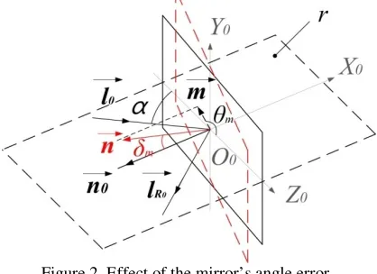
Reflection is a common phenomenon in optical systems. Crooked mirrors will also introduce structural error. The angle error of the mirror will be discussed at first.
In order to describe the crooked mirror, we create a reference coordinate system X0Y0Z0 on the ideal
mirror as shown in Fig 2. X0 axis is perpendicular to
the mirror and Y0 is perpendicular to plane r. Angles
θm and δm are used to describe the angle error of the
mirror. Similarly, δm is the angle between the normal
vector of the ideal mirror n0 and the actual mirror n
and θm is the angle rotating around X0 axis from Z0
axis to vector m which is the projection of vector n
in plane Y0O0Z0. θm describes the direction of the
deviation.
Figure 2. Effect of the mirror’s angle error.
As the linear equation of the incident light is known, its reflected light from the ideal mirror and the actual mirror can be calculated according to law of reflection. The angle between two reflected light beams is γ and its cosine value can be written as
2 2 2 2
cosγ=cos2 sinδm α+(1 2sin− δmcos θm)cos α (4)
Where α is the angle between the light beam and the mirror plane.
Generally speaking, angle precision of the mirror is guaranteed by its mounting surface whose deviation angle can be limited by geometric tolerance but deviation direction can’t be controlled. When calculating error, we take the maximum of the deviation angle as a result. As shown in Equ.5, the deviation angle take the maximum only when angle θm is π and the maximum is
2
mγ
=
δ
(5)At this point, the normal vector of the actual mirror is in the same plane as the incident light.
[image:2.612.331.540.307.459.2]2.4 Reflection mapping
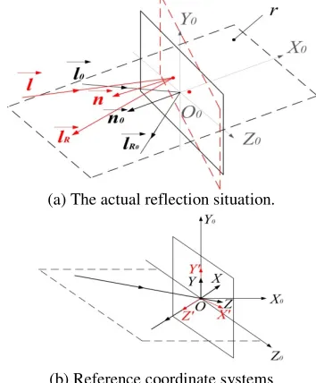
Reflection mappings are used to describe the change of the reflected light beam due to the position and angle error of the incident light and the mirror.
The actual reflection situation is shown in Fig 3(a). The actual reflected light beam lR deviates from
the ideal reflected light beam lR0 due to the error of
the incident light and the mirror. In the reflection, we create three coordinate systems (XYZ、X'Y'Z'
and X0Y0Z0) at the reflection point O shown in Fig
3(b). The relation of these coordinate systems can be established by rotation transformation and they are used to solve the optical vector of the actual light beam.
(a) The actual reflection situation.
[image:3.612.86.263.212.426.2](b) Reference coordinate systems
Figure 3. Schematic diagram of reflection mapping.
The linear equation of the incident light in XYZ
and the plane equation of the actual mirror in X0Y0Z0
are known, according to law of reflection we can get the linear equation of the reflection light in X'Y'Z'
and the position of the reflected light can be written as
sin(2 cos 2 cos 2 )
'
cos( 2 )sin( cos )
sin( cos 2 cos )cos
cos( 2 )sin( cos )
sin sin(2 2 ) '
sin( cos )cos( 2 )
sin cos
[tan( 2 )cos( cos 2 ) sin ]
sin( cos )
m
A m
m m A
m
m
A A m
m
A m
x u
x
y y u
x
δ θ δ θ α
δ δ δ θ α
δ θ δ θ α δ
δ δ δ θ α
θ δ δ
δ θ α δ δ
θ α
δ δ δ θ α δ
δ θ α
+ +
=
+ +
+ +
−
+ +
+ = +
+ +
− + + +
+
(6)
Where um is the position error of the mirror in the
normal direction.
For the sake of convenience in the computation, we neglect higher order terms of the error and Equ.6 can be simplified to Equ.7.
' 2 cos
cos
'
A m A
A A
x
u
x
y
y
α
δ
=
−
=
(7)Thus we can get the final formation of the reflection mapping as
[
]
[
]
' ' ' ' '
( )
[ 2 2 cos ]
T
A A
T
M A A
T
m m A A
l x y
R x y
u x y
θ
δ
θ
δ
π
θ
δ
δ
α
=
=
= − + −
ur
(8)
In this way, we can get the final position and the angle error of each light beam anywhere by repeated transition and reflection mappings. The error introduced by components such as polarization beam splitter (PBS) and beam splitter (BS) can also be
calculated. By analyzing the whole expression of the final light spot, the structural error introduced by each component can be estimated directly and the length of each part of the light path can be optimized.
3 SIMULATION AND ANALYSIS
3.1 Optical system
We take a two-degrees-of-freedom grating interferometer as an example to carry out analysis and simulation verification. The optical structure of the sensor head is shown in Fig.4. At first, the laser beam is split into a reflected laser beam R and a
transmitted laser beam T after passing a BS and R
beam reflected by Mirror 1 turns into the parallel direction with transmitted laser beam T. These two
laser beams both pass through the center PBS and
are divided into two beams respectively. The R beam
divides into reflected laser beam R-R and transmitted
laser beam R-T while the T beam divides into
[image:3.612.340.528.498.624.2]reflected laser beam T-R and transmitted laser beam T-T.
Figure 4. Schematic of the optical sensor head.
The reflected two beams R-R and T-R are both
S-polarization. QW1 is a quarter-wave plate which is
set 45 °. Thus, T-R beam reflected by M2 passes
through QW1 twice and turns into P-polarization and
passes through PBS. R-R beam is reflected by Mirror
R-T and T-T beam are both P-polarization. They
pass through QW2 which is also set 45°. Then these
two laser beams are both reflected by Mirror 4 and turn into a direction where the scale grating is also in Littrow configuration. They diffract back and pass through QW2 again. Then reflected by the center PBS, beam R-T coincides with R-R and beam T-T
coincides with T-R. These two spots respectively
incident into two homodyne phase resolving structure and the result can be used to calculate the displacement of the grating in two degrees of freedom.
3.2 Calculation
We mainly study the interference fringe composed by T-R and T-T as an example. The parameters of
the optical sensor involved are shown in Fig.5. Using the calculating method above, we are able to calculate the final error of the two light beams at reference plane R.
Figure 5. The parameters of the optical sensor.
The result of T-T beam can be written as
0 0
0 0 0 0 4
( 2 cos ,
sin , , 4 2 )
T T pbs T T
T
T T m pbs
l u x L
y L
θ θ θ δ δ δ
− −
−
= − + +
+ + −
uuur
(9)
Where
0 0 4 4
0 4 4 0 4
( ) (2 4 )
(2 4 ) ( 4 2 )
T T l bs bs pbs m pbs m
m m gra m pbs pbs R
L L L L
L L
δ δ δ
δ δ δ δ δ
− − − −
− →
= + + +
+ + + + −
(10)
The result of T-R beam can be written as
0 0
0 0 0 0 2
( 2 cos ,
sin , , 2 2 )
T R pbs T R
T
T R pbs m
l u x L
y L
θ
θ θ δ δ δ
− −
−
= − + +
+ + +
uuur
(11)
Where
0 0 2
0 2 2
( ) ( 2 )
( 2 2 )( )
T R l bs bs pbs pbs pbs m
pbs m pbs m pbs R
L L L L
L L
δ δ δ
δ δ δ
− − − −
− −
= + + +
+ + + +
(12)
This result can be used to calculate and analyze the error of the light beam caused by each component.
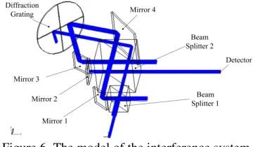
3.3 Simulation verification
Figure.6 shows a photograph of the model established in simulation software. As the polarization status doesn’t affect the calculation, we use another BS to replace the center PBS and QW1
and QW2 are removed.
Figure 6. The model of the interference system.
[image:4.612.344.524.36.141.2]The parameters of the optical system mentioned above are given in Table.1 and the error of each component we set is given in Table.2.
Table 1. Parameters of the optical system.
______________________________________________ Parameters Length/mm
______________________________________________
Ll-bs 12.00 Lbs-pbs 21.06 Lpbs-m4 54.19 Lm4-gra 58.11 Lpbs-m2 44.33 Lpbs-R 30.00
_____________________________________________
Table 2. Errors of the components set in simulation.
______________________________________________ Component Position Error/mm Angle Error/°
______________________________________________ Laser Souce x0=-0.085 δ0=0.1263
y0=0.122 θ0=118.072 BS ubs=0.141 δbs=0.0983 M1 uM1=-0.094 δM1=0.1674 PBS uPBS=0.034 δPBS=0.0499 M2 uM2=0.204 δM2=0.1504 M3 uM3=-0.147 δM3=0.1343 M4 uM4=0.211 δM4=0.1116
_____________________________________________
Due to the errors of the components, the positions of T-T and T-R beams which are initially at the
[image:4.612.315.535.546.733.2]middle of the detector have changed. As we can see in Equs.9-12, the error introduced by each component can be calculated respectively. So we introduce the error in the simulation by each component and the changes of the light beams in position are recorded, shown in Table 3. The final output of the detector is shown in Figure 7.
Table 3. Calculation and simulation in direction x.
______________________________________________ Component Calculation/mm Simulation/mm ____________ _____________ T-R T-T T-R T-T
______________________________________________ Laser Souce -0.2424 -0.3834 -0.2404 -0.3759
PBS -0.1453 -0.0727 -0.1448 -0.0666 M2 -0.1836 0 -0.1862 0 M4 0 -0.5217 0 -0.497
Total -0.5713 -0.9778 -0.5714 -0.9395 _____________________________________________
Calculation and simulation in direction y
______________________________________________ Component Calculation/mm Simulation/mm ____________ _____________ T-R T-T T-R T-T
______________________________________________ Laser Souce 0.4171 0.6815 0.4241 0.6753
PBS 0.1824 -0.0461 0.1754 -0.0273 M2 0.3443 0 0.3364 0 M4 0 0.9783 0 0.987
Total 0.9438 1.6137 0.9359 1.635 _____________________________________________
Figure 7. Final output of the detector.
The coordinate system XOY in the simulation is
different from our reference coordinate system
x0o0y0. Their coordinate axes are just reversed.
Computations indicate that the results from analysis formula are consistent with our simulations.
The result above can also be used to analyze and optimize the optical structure. For example, the angle of the laser source will change the position of
beam T-T and T-R respectively which will make
them separated from each another and reduce the contrast of the final interference signal. This separated distance can be calculated, shown in Equ.13.
0 2 4 4
2 ( pbs m pbs m m gra)
D=
δ
L − −L − −L − (13) By choosing reasonable parameters, the separation caused by the laser source can be eliminated which will improve the interference signal.4 EXPERIMENT
With the above analysis method as a guide, we designed an experimental setup of the two-degrees-of-freedom grating interferometer. A photograph of the experimental setup we built is shown in Fig 8 and its parameters are the same with those in the simulation.
Figure 8. A photograph of the experimental setup.
All the components were processed in designed precision and the final performance was proved to be well. We also performed a preliminary validation experiment. The initial interference fringes of the experimental setup is shown in Figure 9(a). After rotating Mirror 2 for about 0.12°, it changed to Figure 9(b).
(a) Photograph of the initial interference fringes (b) Photograph of the interference fringes Figure 9. A photograph of experimental setup.
This process can be calculated and done in simulation. The change of the interference fringes in simulation is shown in Fig.10.
(a) Simulation result of the initial interference fringes (b) Simulation result of the interference fringes Figure 10. Simulation result of the experiment situation.
As we can see, the experiment result basically matches the result of the simulation and the calculation. Further study on this calculating method will be done in the future.
5 CONCLUSION
We presented a new method of calculating structural error in interferometer measuring system. The method can facilitate the design of the experimental setup of optical configurations and can be used to analyze the structural error of each component. Preliminary simulation and validation have been carried out and the results matched with each other basically. Further study on this method will be done in the future.
REFERENCES
[1].Chih-Kung, L., Chyan-Chyi, W., et al. (2004). Design and construction of linear laser encoders that possess high tolerance of mechanical runout. Applied Optics, 43(31), pp. 5754-5762.
[2].Jin Hui, S., Chun Ying, G., & Zheng Ping, W. (2009). Design and analysis of metal-dielectric nonpolarizing beam splitters in a glass cube. Applied Optics, 48(18), 3385-90. [3].Hung-Lin, H., & Su-Wen, P. (2015). Development of a
grating-based interferometer for six-degree-of-freedom displacement and angle measurements. Optics Express, 23(3), 2451-2465.
[4].Kimura, A., Wei, G., Arai, Y., & Zeng, L. (2010). Design and construction of a two-degree-of-freedom linear encoder for nanometric measurement of stage position and straightness. Precision Engineering, 34(1), 145-155. [5].Liu, C. H., & Cheng, C. H. (2012). Development of a