NEW MODEL TRANSFORMATION USING REQUIREMENT TRACEBILITY FROM REQUIREMENT TO UML BEHAVIORAL DESIGN

(1)

Journal of Theoretical and Applied Information Technology 31st March 2013. Vol. 49 No.3

ISSN: 1992-8645 www.jatit.org E-ISSN: 1817-3195

HETEROGENEOUS MULTI-SENSOR JOINT TRACKING OF

TARGET BURIED IN AEW RADAR BLIND DOPPLER ZONE

YING FU1,2 , ZIYUE TANG1 , YONGJIAN SUN1,3

1 Air Force Early Warning Academy, Wuhan, 430019,China 2 95333 PLA troops，Changsha 410114，China 3 Beijing Institute of Radio Measurement, Beijing, 100854,China

Email: [email protected]

ABSTRACT

Due to adopting the pulse Doppler (PD) system, the blind Doppler zone (BDZ) of airborne early warning (AEW) radar is inevitable. This paper focuses on finding a technique with good estimation performance for tracking airborne targets flying in AEW BDZ. Consequently, combining with interacting multiple models (IMM), extended Kalman filter (EKF) and particle filter (PF), the radar and electronic support measure (ESM) joint tracking BDZ target technique based on IMMEPF is put forward. The advantage of IMM algorithm is not only error reduction but also model prediction. As far as the nonlinear, non-Gaussian problem is concerned, Particle filter is adept usually. For the purpose of overcoming the particle degeneracy phenomenon, it relies on EKF state estimation to generate new particle set. The numerical simulation results justify that the proposed technique shows high precision performance of tracking target buried in BDZ.

Keywords: Heterogeneous Multi-Sensor, Joint Target Tracking, AEW Radar, Blind Doppler Zone,

Interacting Multiple Model, Extended Kalman Particle Filter

1. INTRODUCTION

When AEW radar is operated in air surveillance mode, a target’s return is often buried in the blind Doppler zone which leads to a phenomenon of target plots temporal vanishing or tracks reduplicative initializing. A track derived from same target maybe split into several discontinuous segments. Undoubtedly, this phenomenon results in the decline of the radar intelligence quality. Because AEW radar adopts the PD technology, the existence of BDZ problem is inherent and inevitable [1,2,3,4]. Therefore, the targets buried in the BDZ will be suppressed in company with the clutter and the ground moving targets with low radial speed.

In most cases, active and passive sensors are mutually independent or complementary to detection and tracking. Aimed at the above problem, this paper presents a method of joint tracking BDZ target by radar and ESM. When the target is out of BDZ, the radar and ESM track it together. As long as the target is buried in BDZ, there are ESM measurements only and the ESM will track it alone until it travels out of the BDZ.

(2)

The rest of the paper is organized as follows: Section II quickly previews Target Doppler shift fundamentals and statement of the problem. Section III introduces the IMMEPF algorithm when it is applied to tracking targets buried in BDZ. Numerical examples and conclusion are given in Section IV and V respectively.

2. FUNDAMENTALS AND STATEMENT OF

THE PROBLEM

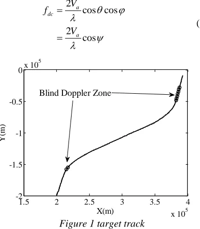
2.1Target Doppler shift and BDZ

The Doppler shift of moving targets relative to the AEW radar is expressed as

(

)

2 _acos _tcos

d

V V

f ψ β

λ +

= (1) Because of the rapid motion of the radar with its platform, some stationary targets, such as the ground and the sea, are sure to generate Doppler shift, which is given by

2

cos cos 2

cos

a dc

a

V f

V

θ ϕ

λ ψ λ =

=

(2)

1.5 2 2.5 3 3.5 4 x 105 -2

-1.5 -1 -0.5

0x 10

5

X(m)

Y

(m

)

[image:2.612.94.291.346.572.2]

Blind Doppler Zone

Figure 1 target track

Where Va and Vt are the flying speed of AEW

and target respectively. ψ is the angle between the course of AEW and the line of sight of radar. β is the angle of the course of target and the line of sight of radar. θ and ϕ are the azimuth angle and the elevation angle of the AEW radar beam respectively. Hdenotes the altitude of the platform.

R is the slant range from the platform to a clutter patch.

The target track is given in Figure 1. It can be learned that the radar will lose the target plots

continuously if fd − fdc∈ Ω where

{

fdt fdt [ fT,fT]

}

Ω = ∈ − denote the BDZ space. In the whole flight process, the target intends to make two BDZs as indicated.

2.2Target and sensor modelling

Figure 2 the geometry of AEW and target

[image:2.612.327.523.606.715.2]

According to

Figure 2, suppose that the radar and ESM are mounted on the same platform. The constant velocity (CV) and constant acceleration (CA) modes are most commonly considered to build models. In this paper, these two models are used. The state space equation is given by

1 1 1

k = k− k− + k k−

X F X G W (3)

X is the state vector of a target defined as

T

[x x x y y y]

=

X    

where x and y denote the target position.,

W signifies process noise, which is zero-mean, white, and Gaussian with covarianceQ(k).

The state transition matrices and the noise gain matrices for each mode can be written in the following forms:

1 1

1 0 0 0 0 0 0

0 1 0 0 0 0 0 0

0 0 0 0 0 0 0 0

,

0 0 0 1 0 0 0

0 0 0 0 1 0 0 0

0 0 0 0 0 0 0 0

T

F G

T

   

   

=  = 

   

   

(4)

(3)

2

2 2

2

2 2

1 0.5 0 0 0

0 1 0 0 0

0 0 1 0 0 0

,

0 0 0 1 0.5

0 0 0 0 1

0 0 0 0 0 1

0.5 0 0 1 0 0 0.5 0 0 1 T T T F T T T T T G T T         =                     =             (5)

where subscripts 1 and 2 in equations (4) and

Error! Reference source not found. denote CV mode and CA mode, and Tis the sampling time. Process noise covariance is simplified under the assumption that the process noise variance in each coordinate is equal and constant.

The measurement model of radar can be written as

( )

rk =hr k + k

Z X V (5) In which,

(

) (

)

(

)

(

)

(

) (

)

2 2 2 2

( ) arctan

k A k A

k A

r k r

k A

k k A k k A

k A k A

x x y x

r

y x

h

x x

r

x x x y y x

x x y x

θ     − + −        −      =_{ }=  ₋            ₋ ₊ ₋     ₋ ₊ ₋    X    (6)

That indicates the measurement vector at the moment k . : nx nu nz

r

h ℜ ×ℜ → ℜ is non-linear measurement function of radar. Vis measurement Gaussian noise.

The measurement model of ESM can be written as

( )

ek=he k + k

Z X η (7) In which,

(

)

(

)

(

) (

2

)

2

arctan ( ) k A k A e e k

k k A k k A

e

k A k A

y x

x x

h

y x x x y x

x x y x

θ θ   −     ₋         =_{  }= _ − + −      ₋ ₊ ₋    X _   (8) That indicates the measurement vector of ESM at the moment k. : nx nu nz

e

h ℜ ×ℜ → ℜ is non-linear measurement function of ESM. ηis ESM measurement Gaussian noise.

3. IMMEPF ALGORITHM

3.1 EKF particle filter

Particle filter is put forward by Gordon foremost. The filter algorithm is not limited by model linear, Gauss hypothesis. It is applicable to any non-linear non-gauss dynamic system.

Standard particle filter algorithm is presented as follows:

(1)Initialization: for k=0;

Set up initial state particle set

{

( )0 0( )

}

1 , N i i i w = X

according to prior distribution of statep X

( )

0 , in

which 0( )

1

i

w N

= ;

(2)for k=1, 2,,T , T is the length of measurement set.

(a)Sampling: get new particle set

{ }

( )

1

N i k

i=

X from sampling state transition probability density function

(

( ) ( )1

)

i i k k

p X X ₋ .

(b)Calculating the weight w_k( )i of the particle

( )i k

X according to the equation

( ) ( ) ( )

( ) ( ) 1

1 ( ) ( )

1 1:

( | ) ( | )

( | , )

i i i

i i k k k k

k k i i

k k k

p p

q

− −

−

ω = ω Z X X X

X X Z , and

normalization ( )

( ) ( ) 1 i i k k N i k j w w w = =

∑

 

. In which,

( )

( k| ki )

p Z X can be got from measurement equation, and ( ( )| ( )1)

i i k k

p X X ₋ can be confirmed by system equation. When measurement noise and system noise are both Gaussian distributed, the expression are as follows respectively.

/ 2

( ) 1/ 2

1

( | ) (2 ) | |

1

exp ( ) ( )

2 z n i k k T i i

k k k k

p

h h

p − −

−

=

 _ _ _ _ ⋅ − _ − _ _ − _

 

Z X R

(4)

/ 2

( ) ( ) 1/ 2

1

( | ) (2 ) | |

1

exp ( ) ( )

2

x n i i

k k

T

i i i i

k k k k

p

f f

p − −

−

=

 _ _ _ _

⋅ − _ − _ _ − _

 

X X Q

X X Q X X

(10) In which, R is the error variance matrix of measurement, Q is the error variance matrix of system.

(3)Output of state estimation: ( ) ( )

1

ˆ N i i

k k k

i

w =

=

∑

X X ;

(4)Resampling:

resample N particles

{ }

( )

1

N i k

i=

X from particle

set

{

( ) ( )

}

1

, N

i i k k

i

w =

X according to the weight w( )ki of

particles, and let w( )ki 1

N

= , then get the new particle set ( )

1

1 ,

N i k

i

N =

 

 

X  .

In standard particle filter, the important probability density function is given as

( ) ( ) ( ) ( )

1 1: 1

( i | i , ) ( i | i )

k k k k k

q X X ₋ Z = p X X ₋ (11) Hence, ( ) ( ) ( )

1 ( | )

i i i

k k− p k k

ω = ω Z X , which has no

consideration of the latest measurements and simplified evaluating weights into calculating likelihoods.

And what’s more, after a few iterations of prediction, it may leads to degeneracy. Removing small weight particles and duplicating the big weight particles by way of resampling in order to reduce the degeneracy effect. Because generation of particle set relies on proposal distribution, the ultimate goal is to make the proposal distribution close to the posterior probability distribution as far as possible, no matter what method is used. Subsequently, the key point of relieving the degeneracy phenomenon is to choose a suitable proposal distribution function.

Since the EKF is an MMSE estimator, its state estimation X( )ki and covariance matrix

( )i k

P of each particle at the moment kcan be utilized to generate new particle set.

( )*

(

( ) ( )

)

~ ,

i i i

k N k k

X X P (12) The proposal distribution is expressed as

( )

( )* ( ) ( ) ( )* ( ) / 2

( ) ( ) 1/ 2

1 1:

1

( | , ) (2 ) | |

1 exp

2

x i

n i i

k k k k

T

i i i i i

k k k k k

q − p − −

−

=

 _ _ _ _

⋅ _− _ − _ _ − __

   

 

X X Z P

X X P X X

(13)

3.2 IMMEPF algorithm

The main idea of the IMM algorithm is to weigh the estimates from the filters matched to the different models. Different models have different state space models. The weights are based on the time variant mode probabilities that imply how close the estimate from each filter is to the corresponding model. Since the IMM algorithm mixes the estimates from different models instead of choosing which mode is true in each time step, it is called a soft switching algorithm, which does not include hard decisions.

To improve the estimation accuracy of IMM, the EKF is introduced and the nonlinear manoeuvring model are used in this paper. Particles in each model are randomly sampled from the prior. Then, they are interacted and updated by model matched EKF . After that they are resampled to be optimized. Finally, particles are combined. This algorithm has high estimation accuracy and immunes to nonlinear and non-Gaussian problems.

Prediction and estimation accuracy are effectively improved by the fixed multiple models and EKF algorithm. The IMMEPF has the following main steps:

(1) Sample the particles randomly: At the moment k, particle set of each model are randomly sampled according to mean value and variance of state variable. The particle number is N. Suppose particle state and covariance of each random sampled particle of m models respectively as

( )

ˆn j

x k and Pˆjn

( )

k .where

1, 2, ,

n=  N,j=1, 2,,m.

(2)Input mixing: Input mixing for corresponding particles of each model, when predict probability of model is

( )

1

m ij i ij i i j

i

k k k

m p m p m

=

∑

and then

( )

( ) ( )

1

ˆ

m

n n

j j i j

i

x k x k m k

=

(5)

( )

{

( )

}

1 ˆ _ˆ ˆ m

n n n n

j i j j j j

i

T

n n

j j

P k k P k x k x k

x k x k

m =   = +_ − _  −   

∑

(15)

(

)

(

)

1 1 1 1 N n n

P k P k

N =

+ =

∑

+ (16) (3)Model-matched EKF filter:

Put particles

{

xnj

( )

k ,Pjn

( )

k ,n=1, 2,,N

}

into EKF which based on the jth model, update state at the moment k+1, the state variable of the nthis

(

1

)

n j

x k+ and its covariance is Pjn

(

k+1

)

, likelihood function is n

(

1

)

j k

Λ + ,and the

corresponding weight is Wjn

(

k+1

)

. Compute the Jacobians ( ),

i k j

H of the measurement models. ( )

(

)

(

)

2 ,1

2 4 2

2 2 2 4 0 0 2 0 0 2 k i rk k

k k k k k k

k k

k k k k k

x r

y r

y r x x y y x r y r

y r

x r

xr y x y y x r x r

  = − _ _ − − −        − − −  _    H       (17) ( )

(

)

(

)

2 ,2

2 4 2

2 2 2 4 0 0 0 0 2 0 0 0 0 0 2 0 k i rk k

k k k k k k

k k

k k k k k

x r

y r

y r x x y y x r y r

y r

x r

xr y x y y x r x r

  = −   − −  −        − − −  _    H       (18) ( )

(

)

(

)

2

,1 2 3

2 2 3 0 0 k i ek

k k k k k k k

k

k k k k k k k

y r

x r x x x y y r x r

x r

x r x x x y y r y r

 − =   − +        − +      H       (19) ( )

(

)

(

)

2

,2 2 3

2 2 3 0 0 0 0 0 0 k i ek

k k k k k k k

k

k k k k k k k

y r

x r x x x y y r x r

x r

x r x x x y y r y r

 − =   − +        − +  _    H       (20) Identify whether the target Doppler shift

d dc

f − f ∈ Ω or not. If fd− fdc∉ Ω,

( ) ( ) ( )

,1 ,1; ,1

i i i

k =  rk ek 

H H H (21)

( ) ( ) ( )

,2 ,2; ,2

i i i

k =  rk ek 

H H H (22)

[ ; ]

k = rk ek

Z Z Z (23)

( )

(

)

(

( )

)

(

( )

)

, 1 , 1 ; , 1

i i i

k k k rk k k ek k k

h X ₋ = h X ₋ h X ₋ _ (24) If fd − fdc∈ Ω,

( ) ( )

,1 ,1

i i

k = ek

H H (25)

( ) ( )

,2 ,2

i i

k = ek

H H (26)

k = ek

Z Z (27)

( )

(

)

(

( )

)

, 1 , 1

i i

k k k ek k k

h X − =h X − (28)

Update the states with EKF:

( ) ( )

, 1 ˆ 1

i i

k k− = k−

X FX

( ) ( ) ( )

, 1 ˆ 1

i i T i T

k k− = k k− k +Gk kGk

P H P H Q

( ) ( ) ( ) ( ) ( ) 1

, 1 , 1

i T i i i T i k k k k k k k k k

−

−  − 

= _ + _

K P H H P H R

( ) ( )

(

( )

)

, 1 , 1

i i i

k = k k− + k k−hk k k− 

X X K Z X

( ) ( ) ( )

, 1

i i i

k = − k k  k k−

P I K H P

(4) Resampling: Evaluate the importance weights of the particles in each model to resample particles, which produce a new set of optimized particles with the same weights.

(5)Update model probability:

(6)

(29)

in which

( )

1

m

n n

j ij j j

c p m k

=

∑

.

(6)Output combination: Combing the corresponding particle set of m models and sum all the particles with the weights to obtain the mean and covariance of the state x k

(

+1

)

and P k

(

+1

)

at the next momentk+1.

(

)

(

) (

)

1

1 1 1

m

n n n

j j

j

x k x k m k

=

+ =

∑

+ + (30)

(

)

(

)

1

1 1

N n n

x k x k

N =

+ =

∑

+ (31)

(

)

{

(

) (

)

(

) (

)

}

1 , 1

1

1 1 1

1 1

m

n n n n

k j j k j

j

T n

j

P k P x k x k

x k x k

m

+ +

=

 

= + +_ + − + _

 + − + 

 

∑

(32)

4. NUMERICAL EXAMPLES

In this section, we show the merits of the IMMEPF algorithm when it is applied to tracking targets buried in BDZ.

Suppose that the simulation system is composed of radar and ESM. And they are mounted on the same platform. Let the radar and ESM sampling interval is one second respectively. The radar is operated at λ =0.23m . The process noises areσx =σy =0.01m. The error statistics for radar measurements are given in terms of the range standard deviation σ =_r 100m ,bearing standard deviation σ =rθ 0.003rad ,range-rate standard deviationσ =r 10m s⋅ -1.The error statistics for ESM measurements are given in terms of the bearing standard deviation σ =eθ 0.005rad , bearing-rate standard deviationσ =_θ 0.001rad s⋅ -1.The limit of

BDZ is -1

0 46m s

L = ⋅ . The number of particle M is 50. The model sequence is assumed to be a first order Markov chain with transition probabilities:

0.96 0.04 0.04 0.96

ij

P =  _

  (33)

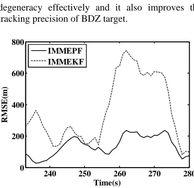
For comparison, the results of tracking targets in BDZ using IMMEKF are presented to evaluate the performance. The root means square error which is

used as index to gauge tracking performance and defined as

( ) ( ) 2 ( ) ( ) 2

1

ˆ ˆ

1 RMSPE

2

N

t t

i

x i x i y i y i

N =

− + −

   

   

=

∑

(34) where N=100is the Monte Carlo simulation times, x iˆ

( )

and y it

( )

are the filter position

estimations at time index k in _ith

Monte Carlo simulation.

0 50 100 150 200 250 300

0 0.2 0.4 0.6 0.8 1

Time(s)

tr

a

ns

it

io

n pr

o

ba

bi

li

ty

CV model CA model

Figure 3 Model Probability

3.855 3.86 3.865 3.87 3.875 3.88

x 105 -3.4

-3.2 -3 -2.8 -2.6

x 104

X(m)

Y

(m)

IMMEPF IMMEKF

[image:6.612.87.531.62.582.2]

Blind Doppler Zone Particles

Figure 4 Tracking target in BDZ

[image:6.612.315.524.236.589.2]

(7)

degeneracy effectively and it also improves the tracking precision of BDZ target.

240 250 260 270 280

0 200 400 600 800

Time(s)

R

M

S

E

(m)

[image:7.612.92.291.92.285.2]

IMMEPF IMMEKF

Figure 5 RMSE position errors versus time

5. CONCLUSION

Focusing on the BDZ target tracking problem, the IMMEPF algorithm is brought forth based on combining the active and passive sensors. Simulation results prove that the advanced technique has outstanding tracking performance. The tracking precision of IMMEPF algorithm is higher than that of IMMEKF algorithm. IMM, EKF and PF can cooperate to provide the optimal estimates and be capable of adaptively handling the manoeuvring motions. The proposal distribution which provided by EKF is effective in reducing the particle degeneracy and improve the tracking precision. This paper turns to a single target tracking problem. However, in many cases, the IMM algorithm is commonly used in multi target tracking. So the future work should be extended to the multiple BDZ targets tracking with multiple sensors by using IMMEPF algorithm.

REFRENCES

[1] J.M.C. Clark, P.A. Kountouriotis,and R.B. Vinter, “A Methodology for Incorporating the Doppler Blind Zone in Target Tracking Algorithms”[C], The 13th International Conference on Information Fusion Proceedings,July 2010, pp.1481-1488.

[2] Farina, A.,”Application of Knowledge-Based Techniques to Tracking Function”[J]. In Knowledge-Based Radar Signal and Data Processing, 2006, (pp. 6-1 – 6-34).

[3] Z.G.Shi, S.H.Hong, and K.S.Chen “Tracking Airborne Targets Hidden in Blind Doppler using current statistical model particle

filter”[J], Progress In Electromagnetics Research, PIER ,82, 2008 , pp.227–240.

[4] N.Gordon and B. Ristic, “Tracking airborne targets occasionally hidden in the blind Doppler,” Digital Signal Processing 12, 2002, pp. 383–393.

[5] F. L. Lewis. “Optimal Estimation”. John Wiley & Sons, Inc., New York, 1986.

[6] Julier.S.J, “The Scaled Unscented Transformation”[C]. Proceedings of the 2002 American Control Conference, May 2002,pp. 4555 - 4559.

[7] BLOM, H. A. P. and Bar-Shalom, Y., “The Interacting Multiple Model Algorithm for Systems with Markovian Switching Coefficient,” IEEE Transactions on Automatics Control, AC-33, 1988, pp. 780–783.

[8] K. Okuma, A. Taleghani, N. de Freitas, J. Little and D. Lowe. “A Boosted Particle Filter: Multitarget Detection and Tracking,” in Proc. European Conf. Computer Vision, 2004, pp.28-39.

[9] Ristic, B., Arulampalam, S., and Gordon, N., “Beyond the Kalman filter: particle filters for tracking applications”[M], Artech House, Norwell, Massachusetts, 2004.