773
COMPUTER SIMULATION AND MODELING OF SHOT
PUTTING PROJECT IN TRACK AND FIELD EVENTS
CAIPING WANG
Taiyuan Normal University, Taiyuan 030012, Shanxi, China E-mail: [email protected]
ABSTRACT
Shot putting is an important component of track and field events and the throwing distance (s, m) is the greatest concern of coaches and athletes. There are mainly three major factors affecting throwing distance: the initial velocity (v, m/s), release angle (A, °) and release height (h, m) in shot push. So far, it is common to use the physical kinematics knowledge in the research of shot putting, but the release height’s impact on the throwing distance is rarely considered. By mathematical modeling and computer simulation, this article analyzes the relation between the three factors (v, A, h) with the throwing distance (s) and determine the best release angle with regard to different release velocity. In addition, the impact of release velocity and release angle on throwing scores is discussed. This article is of certain theoretical guiding significance for athletes and coaches in the selection, training and competition for athletes.
Keywords: Shot Putting, Throwing Distance, Release Angle, Sensitivity
1. INTRODUCTION
In shot putting race, athletes (male) are required to throw the shot (weight, 7.265kg) in a
34.92sartorial area from a circle (d, 2,135m), as
shown in Figure 1[1-3]. The observation of athletes’ video show that their release angles change greatly, which ranges from380 −450. And some is as high
as550[1-6]. Then how to achieve a farther throwing
[image:1.612.122.270.596.672.2]distance? Aiming at to realize the farthest throwing distance, the indexes as the shot’s release height, residence time in the air and the shot’s velocity in horizontal direction are needed. The residence time in the air after the shot-put can be divided into two parts: the first phase is the upward accelerated movement in the vertical direction after shot-put; the second phase is the downward free falling to the grounding [7-10]. This study builds a model, discussing the following questions:
Figure 1: The area of shot putting
Build a mathematical model for shot putting, with release velocity, release angle and release height as parameters [1].
Based on the model, determine the best release angle under different release velocity, with a constant release height. Compare the throwing results’ sensitivity to release angle and release velocity.
2. MODEL HYPOTHESIS
The height of athlete (h) and shot-put release velocity (v) are fixed. The shot reaches the maximum height att1after the shot-put. At t2after
the shot-put, the shot falls to the ground with an acceleration of gravity of g=9.8ms2 . The angle
between the release velocity and horizontal direction isθ , (0≤θ≤90°)(the release angle), the distance between the shot’s drop location and the athlete is the throwing distance S[11-14].
As air resistance has little impact on the shot’s movement, the influence is ignored.
3. SYMBOL DEFINITION
h:The height of the athlete, assuming as 1.7m;
v
:The release velocity of shot putting;θ
:The angle between release velocity and horizontal direction;S
:The distance between shot drop location and the athlete;g
:Acceleration of gravity 28 . 9 m s
774
1
t
:At
t
1 after shot-put, the shot reaches themaximum height;
2
t
:Att
2 after shot-put, the shot falls to theground.
4. MODELING AND SOLVING
4.1. Shot motion trajectory graphic
[image:2.612.103.529.426.714.2]After the shot-put, the trajectory of the shot’s motion is shown in Figure 2.
Figure 2: Shot motion trajectory graphic
4.2. The throwing distance S can be determined through the shot motion trajectory
From the simulated shot motion trajectory graphic, att1, the shot reaches to the highest height
and the velocity at the vertical direction is 0.
∴
v
sin
θ
=
gt
1, I.E. gv t1 = sinθ
∴the maximum height:
g v h gt h t H 2 sin 2 1 ) ( 2 2 2 1 1
θ
+ = + =Then establish the parabolic equation:
g v h g v t a t H 2 sin ) sin ( ) ( 2 2 2 θ
θ + +
− = ∵ h g v h g v a
H = + + =
2 sin sin ) 0 ( 2 2 2 2
2 θ θ
∴
2
g
a
=
−
∴ g v h g v t g t H 2 sin ) sin ( 2 ) ( 2 2 2
θ
θ
+ +− − =
0
)
(
t
2=
H
∴ g v g v g ht 2 sin2 θ sinθ
2 2
2 = + +
∵
S
=
v
cos
t
2The distance between the droop location and the athlete under a constant release height can be determined: g v g v g hv S 2 2 sin ) 2 2 sin ( cos 2 2 2 2 2
2 θ θ θ
+ +
=
4.3. The solving of
θ
corresponding to the largestS
Judging from the ultimate equation of
S
, the throwing distance for a athlete with certain ability (the release velocity), is only related to the release angleθ
. To determine whether there is a maximumS
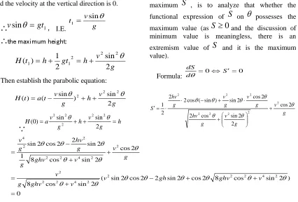
, is to analyze that whether the functional expression ofS
onθ
possesses the maximum value (asS
≥
0
and the discussion of minimum value is meaningless, there is an extremism value ofS
and it is the maximum value).775 i.e.:
0 2 sin 2 2 sin cos 8 2 cos 2 cos 2
sin 2 2 4 2
2 θ θ+ θ θ+ θ− θ=
gh v
ghv v
θ θ
θ
θ sin2 ) 8 cos sin 2 2
tan 2
( 2 2 2 2 4 2
v ghv
v
gh − = +
⇒
θ θ
θ
θ 2 2 2
2 2 2
cos 8 2 sin 2 tan 4 2 tan
4g h − ghv = ghv
⇒
θ θ
θ
θ 2 2 2
2
cos 2 2 sin 2 tan 2
tan v v
gh − =
⇒
θ θ
θ θ
θ sin 2 cos2 (cos2 1)cos 2 2
sin2 − 2 2 = 2 + 2
⇒gh v v
] 2 cos 2 cos 2 cos ) 2 cos 1 [( 2
sin2 θ = 2 − 2 θ θ+ 2 θ+ 3 θ
⇒gh v
θ θ
θ) (1 cos2 )cos2
2 cos 1
( − 2 = 2 +
⇒gh v
θ
θ) cos2
2 cos 1
( 2
v
gh − =
⇒
2
2 cos
v gh
gh + =
⇒ θ
Then:
When
2 arccos
2 1
v gh
gh
+ =
θ
, the throwing distance is the farthest.
4.4. The function of
θ
corresponding tov
in modeling result figureAccording to
2 arccos
2 1
v gh
gh
+ =
θ
[image:3.612.324.519.134.305.2], the functional image of
v
corresponding toθ
is shown in Figure 3.Figure 3: The corresponding angle to the largest release velocity with different velocity
As can be seen from Figure 3, the best release angle differs when the release velocity changes. And the best release angle tends to be 0
45 as the
velocity increases continuously.
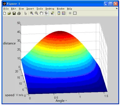
4.5. The computer simulation of shot putting distance’ sensitivity to the release velocity and release angle
[image:3.612.326.519.335.508.2]Figure 4: The throwing distance under different velocity and angle
Figure 5: The derivation of S to
v
under different velocity and angleFigure 6: the derivation of S to the release angle under
[image:3.612.101.297.441.630.2] [image:3.612.324.521.538.695.2]776 Judging from the above three figures (Figure 4, Figure 5, Figure 6.), it is apparently to determine the shot putting distance’ sensitivity to the release velocity and release angle. The influence of release velocity v and release angle A on the throwing distance can be told from the figures, which has certain theoretical guiding significance for the
athletes and coaches in the further training and completion.
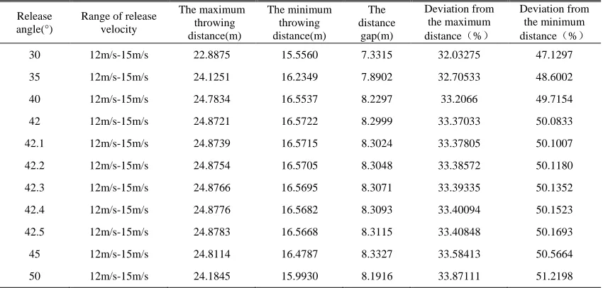
[image:4.612.98.523.208.411.2]By means of Excel software, the calculated throwing distance under different release angle when the release velocity ranges from12m/s to 15m/s (supposing that the release height h=2m) is shown in Table 1.
Table 1: The throwing distance when the release velocity ranges from 12m/s to 15m/s
Release angle(°)
Range of release velocity
The maximum throwing distance(m)
The minimum throwing distance(m)
The distance
gap(m)
Deviation from the maximum distance(%)
Deviation from the minimum distance(%) 30 12m/s-15m/s 22.8875 15.5560 7.3315 32.03275 47.1297 35 12m/s-15m/s 24.1251 16.2349 7.8902 32.70533 48.6002 40 12m/s-15m/s 24.7834 16.5537 8.2297 33.2066 49.7154 42 12m/s-15m/s 24.8721 16.5722 8.2999 33.37033 50.0833 42.1 12m/s-15m/s 24.8739 16.5715 8.3024 33.37805 50.1007 42.2 12m/s-15m/s 24.8754 16.5705 8.3048 33.38572 50.1180 42.3 12m/s-15m/s 24.8766 16.5695 8.3071 33.39335 50.1352 42.4 12m/s-15m/s 24.8776 16.5682 8.3093 33.40094 50.1523 42.5 12m/s-15m/s 24.8783 16.5668 8.3115 33.40848 50.1693 45 12m/s-15m/s 24.8114 16.4787 8.3327 33.58413 50.5664 50 12m/s-15m/s 24.1845 15.9930 8.1916 33.87111 51.2198
As can be seen from Figure 1: under different release angle, the throwing distance gap is huge when the release velocity ranges in 12m/s-15m/s, about 7m-8m, 32%-34% of the maximum throwing distance and 47%-52% of the minimum throwing distance.
[image:4.612.94.524.514.713.2]By means of Excel software, the calculated throwing distance under different release velocity when the release angle ranges from42° to 42.5° (supposing that the release height h=2m) is shown in Table 2.
Table 2: The throwing distance when the release angle ranges from 42°to 42.5°
Release velocity(°)
Range of release angle
The maximum throwing distance(m)
The minimum throwing distance(m)
The distance
gap(m)
Deviation from the maximum distance(%)
Deviation from the minimum distance(%)
777 As can be seen from Figure 2: under different release velocity, the throwing distance gap is small when the release angle ranges from 42° to 42.5°, about 0.001mto0.007m, 0.001%-0.030% of the maximum throwing distance and 0.003%-0.03% of the minimum throwing distance.
By analyzing the above two groups of deviation data, it can be seen that the deviation of release velocity’s impact on the throwing distance is 7-8m, and about 32%-34% of the maximum throwing distance and 47%-52% of the minimum throwing distance. the deviation of release angle’ impact on the throwing distance is 0.001-0.007m, and about 0.001mto0.007m, 0.001%-0.030% of the maximum throwing distance and 0.003%-0.03% of the minimum throwing distance.
As a result, the impact of release velocity on throwing distance is much higher than that of release angle on throwing distance. This result indicates that the main focus should be on increasing the release velocity in the training process.
5. CONCLUSIONS AND SUGGESTIONS
The following conclusions can be reached based on the above model analysis: Within the tolerance range of the best shot angle, for the same athletes, sliding speed is the most important external factor that affects the throwing distance and the second important factor is release height. Therefore, more attention should be paid to the strengthening of the sliding movement and the practice of release velocity. Athlete should choose the best release angle adaptable to oneself based on the specific circumstances, rather than excessive pursuit of the best theory release angle.
REFERENCES:
[1] Li M.X, Yan B.T, Wu T.X. , “The Best Angle of Putting the Shot by Test hypothetical”,
journal of xi’ an institute of physical education, Vol.14, No.3, 1997, pp.89-93.
[2] He W.D. , “The Relations between Shot Put and the Law of Golden Section”, Journal of Guangxi University for Nationalities (Natural Science Edition), Vol.6, No.03, 2000, pp.223-227.
[3] Sun W.B. , “Analysis on the key role of the last strength during the throwing of javelin”,
Journal of Science of Teachers College and University, Vol.24, No.04,2004, pp.55-56.
[4] Li T., “Application of imagery training quantification of back gliding shot in teaching ”, Journal of Shandong Normal University (Natural Science), Vol.16, No.04, 2001, pp.473-474.
[5] Xu R.Z. , “The influence of the vaulting foot orientation on the maximal effort in shot putting”, Journal of Yanbian University (Natural Science Edition), Vol.26, No.04, 2000, pp.316-318.
[6] Shao G, Wang Y., “The Application of "Contrary Teaching Method" to Putting the Shot”, Journal of Yunnan Normal University (Natural Sciences Edition), Vol.25, No.05, 2005,pp.75-77.
[7] Zhang Yunliang, Cui Degang, Liu Chunming, “Comparison among performances predictions for 29th Beijing Olympic Games track and field”, Journal of Tianjin Sport College, Vol.23, No.5, 2008, pp.430-432.
[8] Zhang Yunliang, “Prospect of global competitive sport after 29th Beijing Olympic Games”, Journal of Wuhan Sport College, Vol.31, No.1, 2009, pp.4-8.
[9] Gaojie, “Professionalism—real selection for 21st sport teachers education”, Weekly Examination literature forum, Vol.2, 2007, pp.115-116.
[10] Fanqun, “Situation in performance evaluation for managers in colleges and universities and creative analysis”, Modern education science, Vol.4, 2009, pp.73-76.
[11] Liangyu, Liangjuan, “Thinking in performance evaluation for teachers in colleges and universities”, Heilongjiang Education, Vol.11, 2007, pp.85-87.
[12] Li Zhihe, Wu Fengli, Zhang Shengtai, et al., “Example study of performance check for researches in colleges and universities”,
Modern education technology, 2009,8:16-20. [13] Yangbo, Xu Simao, “Thinking in performance
evaluation of sport teachers in colleges and universities”, sport literature search, Vol.18, No.4, 2010, pp.128-131.