SECRET DATA HIDING BY OPTIMIZING GENERAL SMOOTHNESS DIFFERENCE EXPANSION BASED METHOD

CRUDE OIL PREDICTION USING A HYBRID RADIAL BASIS

FUNCTION NETWORK

Dr S. KUMAR CHANDAR #1, Dr. M. SUMATHI#2, Dr S. N. SIVANANDAM #3

#1

PhD SCHOLAR / ASSOCIATE PROFESSOR,

Madurai Kamaraj University, Madurai / Christ University, Bangalore, India

#2

ASSOCIATE PROFESSOR,

Sri Meenakshi Government College For Arts For Women (Autonomous), MADURAI, INDIA

#3

PROFESSOR EMERITUS,

Karpagam College Of Engineering, Coimbatore, India

Email: #[email protected], #[email protected], #[email protected]

Abstract:

In the recent years, the crude oil is one of the most important commodities worldwide. This paper discusses the prediction of crude oil using artificial neural networks techniques. The research data used in this study is from 1st Jan 2000- 31st April 2014. Normally, Crude oil is related with other commodities. Hence, in this study, the commodities like historical data’s of gold prices, Standard & Poor’s 500 stock index (S & P 500) index and foreign exchange rate are considered as inputs for the network. A radial basis function is better than the back propagation network in terms of classification and learning speed. When creating a radial basis functions, the factors like number of radial basis neurons, radial layer’s spread constant are taken into an account. The spread constant is determined using a bio inspired particle swarm optimization algorithm. A hybrid Radial Basis Function is proposed for forecasting the crude oil prices. The accuracy measures like Mean Square Error, Mean Absolute Error, Sum Square Error and Root Mean Square Error are used to access the performance. From the results, it is clear that hybrid radial basis function outperforms the other models.

Keywords: Crude oil prices, Standard & Poor’s 500 Stock Index, hybrid radial basis function, Particle

Swarm Optimization.

1.INTRODUCTION

Crude oil is one of the most important commodities worldwide. The price fluctuation in crude oil is the major concern which affects our economy. The daily fluctuations in the crude oil prices not only affect our financial market, it also affects each individual in the country. Also, the crude oil prices directly affect the petrol prices. Hence, it is essential to forecast the crude oil prices which are helpful for the investors to make decisions based on the energy markets.

In the literature study, the applications of artificial neural networks for predicting the crude oil and its performance are discussed. The soft computing techniques such as Artificial Neural Networks (ANN), Support Vector Machines, Genetic Algorithms, Fuzzy logic are applied for the prediction of future crude oil prices. Among the techniques, Artificial neural networks suits well for the prediction of crude oil.

Wen Xie et al. (2006) [1] proposed a new method for forecasting crude oil prices using support vector machine. The results are compared with ARIMA models and back propagation neural networks and proved that the proposed method outperforms the other two methods. Yejing Bao et al. (2007) [2] proposed discrete wavelet transform based least square support vector machine for forecasting the future crude oil prices. Haidar et al. (2008) [3] presented a three layer feed forward networks for forecasting future prices of crude oil prices up to three days ahead. The inputs considered by the authors are crude oil future prices, dollar index, gold price, oil spot price and S&P 500 index.

proposed multicyclic Hubbert model for forecasting World Crude Oil Production. This model was very simple and accurate than the other methods.

Bashiri Behmiri et al. (2013) [6] presented a wide literature study on crude oil price forecasting. The forecasting methods are grouped into two categories namely quantitative and qualitative. Quantitative methods are divided into time series models, structural models, financial models, computational approach. These models are used to find the numeral future values of oil prices. The qualitative methods are divided into Delphi methods, fuzzy logic in which these methods analyzed the irregular patterns on oil prices.

Lubna A Gabralla et al. (2013) [7] proposed a wide literature on two decades of research on crude oil price forecasting. Mayuree Sompui et al. (2014) [8] proposed an artificial neural network of one, two, three and four hidden layers to forecast the crude oil price direction in short term. Data was collected from Energy Information Administration from the period 2002 to 2013. This proposed method outperforms the least square methods.

2. RESEARCH DATA

Crude oil is related with other commodities like gold price, silver price, stock market, exchange rates etc. The period of the study is 1st January 2000 to 31st April 2014. from This paper uses four commodities like historical data’s of gold prices, Standard & Poor’s 500 stock index, foreign exchange rate for forecasting the future prices of crude oil. The monthly data of these four commodities are collected from 1st January 2000 to 31st April 2014.

The gold price data was collected from the website address http://www.bullion-rates.com/gold/INR/2014-4-history.html, Crude oil data was gathered from the website address

http://www.indexmundi.com/commodities, foreign exchange data was gathered from the website address http://fxtop.com/en/historical-exchange-rates.php?MA=1 and Standard & Poor’s 500 stock index was collected from the website address

http://bseindia.com.

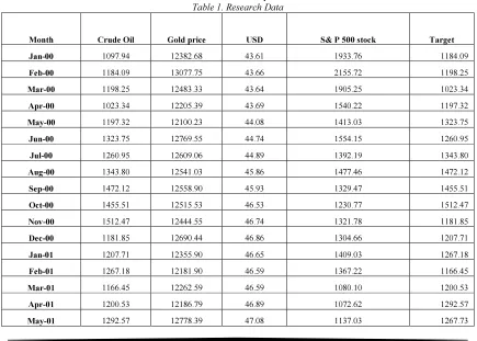
The sample dataset taken for the study is shown in the Table 1. The first column represents the month, the second column represents the monthly average data of crude oil prices, the third column represents the monthly average data of foreign exchange rates, the fourth column denotes the monthly average data of S&P 500 stock index and the last column denotes the actual target crude oil prices.

Table 1. Research Data

Month Crude Oil Gold price USD S& P 500 stock Target

Jan-00 1097.94 12382.68 43.61 1933.76 1184.09

Feb-00 1184.09 13077.75 43.66 2155.72 1198.25

Mar-00 1198.25 12483.33 43.64 1905.25 1023.34

Apr-00 1023.34 12205.39 43.69 1540.22 1197.32

May-00 1197.32 12100.23 44.08 1413.03 1323.75

Jun-00 1323.75 12769.55 44.74 1554.15 1260.95

Jul-00 1260.95 12609.06 44.89 1392.19 1343.80

Aug-00 1343.80 12541.03 45.86 1477.46 1472.12

Sep-00 1472.12 12558.90 45.93 1329.47 1455.51

Oct-00 1455.51 12515.53 46.53 1230.77 1512.47

Nov-00 1512.47 12444.55 46.74 1321.78 1181.85

Dec-00 1181.85 12690.44 46.86 1304.66 1207.71

Jan-01 1207.71 12355.90 46.65 1409.03 1267.18

Feb-01 1267.18 12181.90 46.59 1367.22 1166.45

Mar-01 1166.45 12262.59 46.59 1080.10 1200.53

Apr-01 1200.53 12186.79 46.89 1072.62 1292.57

Jun-01 1267.73 12702.23 47.24 1050.43 1169.12

Jul-01 1169.12 12611.85 47.45 1007.38 1216.33

Aug-01 1216.33 12836.74 47.26 986.25 1192.58

Sep-01 1192.58 13503.83 47.77 850.56 995.46

Oct-01 995.46 13592.68 48.11 902.84 897.07

Nov-01 897.07 13254.95 47.95 1011.26 887.42

Dec-01 887.42 13217.92 47.91 1005.82 925.63

The statistics of the research data is given in Table 2.The maximum, minimum, mean and standard deviation is calculated from the four commodities and is listed below.

Table 2. Statistics of the research data Input data

Max Min Mean Standard

Deviation Crude Oil 6,928.11 887.42 3091.02 1716.68 Gold price 95,194.24 12,100.23 39317.53 26632.32

USD _{63.90 39.26 47.44 5.03}

S&P 500 stock

8,592.43 850.56 4398.48 2500.74

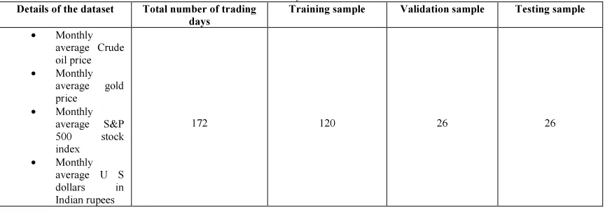
The entire data is divided into training dataset, validation dataset and testing dataset. Totally 172 data from the period (1st January 2000 – 31st April 2014) is retrieved and among that,

training dataset have 120 days (70%) and validation dataset have 26 days (15%) and testing dataset have 26 days (15%). The details of historical dataset are shown in Table 3.

Table 3: Details of Historical dataset Details of the dataset Total number of trading

days

Training sample Validation sample Testing sample

• Monthly average Crude oil price

• Monthly average gold price

• Monthly

average S&P 500 stock index

• Monthly average U S dollars in Indian rupees

172 120 26 26

3. PROPOSED HYBRID RADIAL BASIS

FUNCTION NETWORK

This section explains the overview about Radial Basis Function Network and it explains the proposed hybrid Radial Basis Function Network.

3.1Overview on Radial Basis Function

Network

Radial basis functions network is one type of feed forward networks. It is better than the back propagation network in terms of classification and learning speed. It is a fast learning and powerful

self organized neural network. It was developed by M.J.D. Powell in the year 1980. It has three layers namely input layer, hidden radial basis function nodes layer and output layer. The output nodes form a linear combination of the radial basis functions computed by the hidden layer nodes.

The radial basis function has the form f(x) =

ϕ

(

x

−

µ

)

In this equation, x denotes the input vector,

µ

denotes the Euclidian distance.

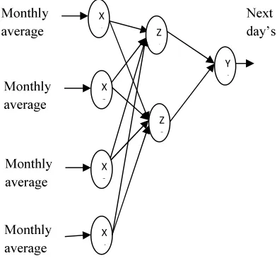
The architecture of the radial basis function is shown in Figure 1. The four parameters such as

monthly average crude oil prices, monthly average of gold prices, monthly average S&P 500 index and monthly average US dollars are given as input to the network. The output of the network gives the next day’s crude oil prices.

Figure 1. Architecture of Radial Basis Function

3.2 Proposed Hybrid Radial basis function When creating a radial basis functions, the factors like number of radial basis neurons, radial layer’s spread constant are taken into an account. Determination of spread constant is a major challenge in the radial basis function network. An inappropriate spread constant will cause overfitting or underfitting of a radial basis function network. When the spread constant is too high, then there will be overfitting of a network and when the spread constant is too low, then there will be underfitting of a network. Choosing an appropriate spread constant will increase the accuracy of the network. The author Hongfa Wang et al. 2013 [9] proposed determination of spread constant of radial basis function using Genetic Algorithm (GA). GA may have the tendency to converge towards local optima (Valle et al. 2008) [10] rather than the global optimum of the problem, if the fitness function is not defined properly. For specific optimization problems, and given the same amount of computation time, simpler optimization algorithms may find better solutions than GA. Operating on dynamic data sets using GA is a difficult task. This paper uses Particle Swarm Optimization for optimizing the spread constant of the radial basis function network to achieve better solutions. Hence, the proposed hybrid radial basis function determines

the suitable spread constant by using Bio-inspired Particle Swarm Optimization algorithm. This section discusses the basic concepts of particle swarm optimization and discusses about the hybrid radial basis function algorithm.

3.2.1 Particle Swarm Optimization

Particle Swarm Optimization (PSO) is an evolutionary computation technique developed by Eberhart and Kennedy (Eberhart et al. 1995, Kennedy et al. 1995) inspired by the social behavior of bird flocking and fish schooling. PSO has its roots in artificial life and social psychology, as well as in Engineering and Computer Science. In addition, PSO uses the swarm intelligence concept, which is the property of a system, whereby the collective behaviors of unsophisticated agents that are interacting locally with their environment create coherent global functional patterns.

PSO utilizes a swarm of particles that fly through the problem hyperspace with given velocities. A particle has the following information to make a suitable change in its position and velocity:

• A global best that is known to all and immediately updated when a new best position is found by any particle in the swarm (

p

X 1

X 2

X 3

Z 1

Z 2

Y 1

X 4 Monthly

average

Monthly average

Monthly average

Monthly average

L

o

o

p

u

n

ti

l

ma

x

im

u

m

it

er

ati

o

n

Start

For each particle’s position (p) evaluate fitness

If fitness (p) better than fitness (

p

i

p

i

Set best of

p

i

p

g

Update particle’s position and velocity

Give

p

g

Lo

o

p

u

n

ti

l

all

p

ar

ti

cle

s

ex

h

a

u

st

Initialize Particle’s position and velocity randomly

Stop • The local best, which is the best

solution that the particle has seen (

p

i

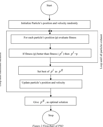
Figure 2 shows the various steps in applying PSO for any optimization problem. PSO maintains a population of particle’s position that represents candidate solutions to the problem.

Each position of particle in the population has an adaptable velocity, according to which the particle moves in the search space. Each position in the population is evaluated to give some measure of its fitness to the problem using the objective function.

Figure 2 Flowchart of PSO

For each iteration the velocities of the individual particles are stochastically adjusted according to the historical best position for the particle itself and the neighborhood best position. Both the particle best and the neighborhood best are derived according to a user defined fitness function. The

movement of each particle naturally evolves an optimal or near-optimal solution.

)

(

)

(

k

wv

c

rand

p

x

c

rand

p

x

v

=

+

−

+

−

(2) i k i k i

k

x

v

x

=

+

v

= velocity of particle i at

iteration k,

i k

v

+ _{= velocity of particle i at iteration}

k+1,

i k

x

= position of particle i at iteration k,

i k

x

1

+ _{= position of particle i at iteration k+1,}

c

self confidence factor,

c

factor,

w

i

p

individual best,

g

k

p

= global best at iteration k. The equation (2) updates the velocity and equation (3) updates the position of the respective particle at the end of iteration. The equation (2) can be viewed as addition of three

components. The first component ‘

i

k

v

’ represents the current motion of the particle, second

component ‘

)

(

i

k

x

i

p

rand

₋

’ represents the particle’s memory influence and finally the third

component ‘

)

(

i

k

x

g

k

p

rand

−

’ represents the swarm’s memory influence.

3.2.2 Fitness Function Formulation

On applying stochastic based optimization algorithms like PSO, the important factor is the formulation of fitness function. Evaluation of the individuals in the population is accomplished by calculating the objective function value for the problem using the parameter set. For forecasting problem under consideration, the key objective is,

• To minimize the mean square error in

each iteration.

The fitness function (Pu) is calculated by the

summation of power of difference between the target values and the output values calculated from the network which is given in equation (4),

Fitness function (Pu) = sum

((Target-Y) ^2) (4)

Here ‘Target’ represents the target crude oil values and ‘Y’ represents the output values generated from the proposed hybrid radial basis network.

3.2.3 Proposed Hybrid Radial Basis Function network algorithm for Crude oil forecasting The algorithm discussed below describes in detail the various steps involved in crude oil forecasting.

Step1: Start the process.

Step2: Read the training data and the testing

data. The entire data is divided into training dataset, validation dataset and testing dataset. Totally 172 data from the period (1st

January 2000 – 31st

April 2014) is retrieved and among that, training dataset have 120 days (70%) and validation dataset have 26 days (15%) and testing dataset have 26 days (15%).

Step 3: Compute the distance‘d’ between the

input pairs using the MATLAB command ‘pdist’ is given in equation (5)

d= pdist (trainingdata)

(5)

Step 4: Compute the maximum distance

among the input pairs using the equation (6)

max_d= max (d)

(6)

Step 5: Invoke Particle Swarm Optimization

algorithm for calculating the spread constants required for radial basis function.

Step 6: Initialize spread constant to some

random values in the range of 0 to max_d. Initialize the swarm position with random spread constant values. Set the number of generations, tuning self confidence factor and swarm

confidence factor

1

c

,

2

c

to start the optimal solution searching.

Step7: Calculate the radial basis function

using the MATLAB command ‘newrb’ with arguments containing trainingdata, targetdata and spreadconstant. Then calculate the output of the network using the equation (8)

net=newrb(trainingdata,target,spr ead)

Y=sim(net,inputs)

(8)

Step8: Evaluate position and velocity of

each particle.

Step9: For each particle evaluate the fitness

function (

P

u

Step10: Update particle individual best (

i

p

),

global best (

g

p

), worst position (pw) in the velocity update equation and obtain the new velocity pertaining to each weight coefficients.

Step11: Update new velocity value from (2)

and obtain the new position of the particle. Find the optimal solution for the updated new velocity and position.

Step12: Stop the process when computation

is done for all the input data and maximum iterations reached. The optimized spread constant values are computed.

4. RESULTS AND DISCUSSIONS

This section presents the results and discussions for forecasting of crude oil using the proposed approach.

4.1 Feed forward networks

A network is said to be feed forward network when the outputs are not directed back as inputs to the same or preceding layer. In this network, the information moves only in one direction and there is no feedback. All the layers are trained using Levenberg-Marquardt (TRAINLM) function and INITNW and TRAINS functions are used for adaptation of weights. The performance measures like mean square error, mean absolute error, sum square error and root mean square error obtained using feed forward networks are listed in the table 4.

4.2 Radial Basis Function Neural network Radial Basis Function Network is a particular type of Feed Forward Network used for approximating the functions and recognizing the patterns. The spread constant is considered to be 1 and the performances measures like mean square error, mean absolute error, sum square error and root mean square error are calculated using radial basis network and it is listed in the table 4.

4.3 Hybrid Radial Basis Function Neural

Network

The proposed approach is tested with 30 independent trials with different values of random seeds and control parameters. The optimal result is obtained for the following settings given below:

• Maximum Iteration : 30 • Swarm Size : 49 • Inertia constant : 1.0

•

1

c

,

2

c

: 0.2, 0.2

The proposed approach is developed using MATLAB R2009 and executed in a PC with Pentium IV processor with 2.40 GHz speed and 256 MB of RAM. With the above settings, outputs for the proposed hybrid radial basis function approach is obtained and compared with the other approaches like feed forward network and radial basis function network.

The following performance indicators are used to predict the output response.

• Mean Square Error (MSE)

• Mean Absolute Error (MAE)

• Sum Squared Error (SSE)

• Root Mean Square Error (RMSE)

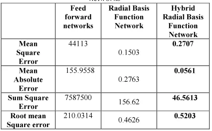
The proposed model is compared with respect to Mean square error, Mean absolute error, Sum squared error and Root mean square error.

Table 4. Performance comparison of different neural networks Feed forward networks Radial Basis Function Network Hybrid Radial Basis Function Network Mean Square Error 44113 0.1503 0.2707 Mean Absolute Error 155.9558 0.2763 0.0561 Sum Square Error

7587500 _156.62 46.5613

Root mean Square error

210.0314

0.4626 0.5203

From the table, it is inferred that error values of feed forward networks are higher when compared to radial basis function network. Using Hybrid radial basis function network, the error values are still reduced when compared to radial basis function network.

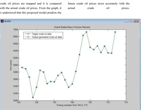
crude oil prices are mapped and it is compared with the actual crude oil prices. From the graph, it is understood that this proposed model predicts the

future crude oil prices more accurately with the

actual crude oil prices.

Figure 3. Comparison graph of Predicted monthly average crude oil prices Vs Target crude oil prices

5. CONCLUSION

This paper proposes a hybrid radial basis function network for forecasting the crude oil prices. Here the determination of spread constants in radial basis neural network is done by using particle swarm optimization. The period of study is taken from 1st

Jan 2000- 31st

Apr 2014. The commodities like historical data’s of gold prices, Standard & Poor’s 500 stock index (S & P 500) index and foreign exchange rate are considered as inputs for the network. The accuracy measures like Mean Square Error, Mean Absolute Error, Sum Square Error and Root Mean Square Error are used to access the performance. From the results, it is clear that hybrid radial basis function outperforms the other models.

REFERENCES

[1] Wen Xie, Lean Yu, Shanying Xu, and Shouyang Wang, A New Method for Crude Oil Price Forecasting Based on Support

Vector Machines, Computational Science – ICCS 2006,Lecture Notes in Computer Science Vol. 994, pp 44-451, 2006.

[2] Yejing Bao, Xun Zhang, Lean Yu, Shouyang Wang, Crude Oil Price Prediction Based On Multi-scale Decomposition, Computational Science – ICCS 2007 Lecture Notes in Computer science Volume 4489, pp 933-936, 2007 .

[3] Imad Haidar, Siddhivinayak Kulkarni, and Heping Pan, Forecasting Model for Crude Oil Prices Based on Artificial Neural Networks, International Conference on Intelligent Sensors, Sensor Networks and Information Processing, pp. 103 – 108, 2008,.

[5] Ibrahim Sami Nashawi, Adel Malallah and Mohammed Al-Bisharah, Forecasting World Crude Oil Production Using Multicyclic Hubbert Model, Energy Fuels, Vol.24, pp. 1788–1800, 2010.

[6] Bashiri Behmiri, Niaz and Pires Manso, José Ramos, Crude Oil Price Forecasting Techniques: A Comprehensive Review of Literature (June 6, 2013).

[7] Lubna A Gabralla, Ajith Abraham, Computational Modeling of Crude Oil Price Forecasting: A Review of Two Decades of Research, International Journal of Computer Information Systems and Industrial Management Applications. ISSN 2150-7988 Volume 5, pp. 729-740, 2013.

[8] Mayuree Sompui and Wullapa

Wongsinlatam, Prediction Model for Crude Oil Price Using Artificial Neural Networks, Applied Mathematical Sciences, Vol. 8, pp. 80, 3953 – 3965, 2014.

[9] Hongfa Wang, Xinai Xu, Determination of Spread Constant in RBF Neural Network by Genetic Algorithm, International Journal of

Advancements in Computing

Technology(IJACT), Vol 5, No.9, pp. 719-726, May 2013.

[10]Valle, Y., Venayagamoorthy, G.K., Mohagheghi, S., Hernandez, J. and Harley, R.G. “Particle Swarm Optimization: Basic Concepts, Variants and Applications in Power Systems”, IEEE Transaction on Evolutionary Computation, Vol.12, No.2, pp.171-195, 2008.

[11]Eberhart, R. and Kennedy, J. “A new optimizer using particle swarm theory,” Proceedings of 6th International Symposium Micro Machine and Human Science (MHS), pp. 39–43, 1995.