Novel Ensemble Neural Network Models for better
Prediction using Variable Input Approach
Basawaraj Gadgay
1, Subhash Kulkarni
2, Chandrasekhar B
31
Dept . of Electronics Engineering, JNTU;
2
JPN College of Engineering, Mahaboobnagar,
3
SRS Institute of Technology, Bangalore
ABSTRACT
In this work, seven Ensemble Artificial Neural Network (ANN) models, namely, Multilayer Perceptron Network (MLPN), Elman Recurrent Neural Network (ERNN), Radial Basis Function Network (RBFN), Hopfield Model (HFM), Ensemble Neural Network based on Variable Inputs with No Hidden Layers (ENN-V-S), Ensemble Neural Network based on Variable Inputs with Hidden Layers (ENN-V-M), Ensemble Neural Network based on Time Inputs with No Hidden Layers (ENN-T-M), are developed to predict the rainfall for one of the large cities of India i.e. Bangalore. Different network models are developed to match the predicted results with the actual data and ENN-Average is found to be the best among all. In order to test this, actual rainfall data was collected in Bangalore city for the calendar years 2007, 2008 and 2009. This data was used as training data for the ANNs and predictions were made for the year 2010. Again these predictions were compared with the actual data to verify the performance of the ANNs. In this study, it has been proved that ENN-Average model based on back propagation algorithm provide better accurate predictions than the SNN and ENN models based on other algorithms.
Keywords:
Artificial Neural Networks, Ensemble Neural Networks, Rainfall Prediction, ENN Averaging.1.
INTRODUCTION
Rainfall amounts vary geographically within India across different cities and also within the city. For example, rainfall characteristics and patterns in the cities like Bangalore and Mumbai are different from that of Chennai and Kolkata. Additionally, spatial variation in rainfall for shorter periods, such as one to five days, is significantly higher than monthly, seasonal and annual rainfall. Hence, in this research work, spatially varying rainfall across Bangalore is considered based on varying meteorologically/climatological conditions during dry and wet periods. Rainfall is treated as a multidimensional process spread over space and time. For a selected rainfall occurrence, different and multiple possible realizations can be formulated that are occurring along the time scale. Average rainfall value over an area of all possible formulations of that occurrence could be considered for the analysis. The availability of rainfall data and its duration are important for hydrologic analysis and design of water resources systems.
2.
LITERTAURE
REVIEW
ASCE (1996), Larson & Peck (1974) and Vieux (2001): The problems of missing data due to a different of reasons are discussed. And, systematic and random errors that occur in the measurement of hydrologic variables is also analyzed.
Vieux (2001): Systematic errors that occur in the rain gage measurements are discussed It is classified as can be of various types: 1) water loss during measurement 2) adhesion loss on the surface of the gage and 3) raindrop splash from the collector 4) Complete lack of data in many situations in situations like the rainfall gage malfunctions for a specific period of time. Other types of errors include errors in recording of rainfall data due to tree growth, problems in instrumentation or techniques used to measure the rainfall amounts. These types’ of errors are very critical since they affect the integrity and continuity of rainfall data. They also ultimately influence the results of and predictions made by hydrologic models that use rainfall as input like artificial neural networks. It is very important to estimate the missing data in many hydrological modeling studies. Interpolation, extrapolation, traditional weighting and data-driven methods are generally used for estimating missing data.
Simanton & Osborn (1980) and Wei & McGuinness (1973): spatial interpolation methods such as inverse-distance non-linear deterministic and stochastic interpolation methods are part of weighting methods. Similarly, regression as well as time series analysis methods belong to data-driven approaches.
The handbook of hydrology (ASCE, 1996): two methods for estimation of missing data, normal-ratio and inverse distance weighting methods are recommended.
Singh and Chowdhury (1986): 13 rainfall estimation methods are analyzed and compared. It is found that isohyetal method yields higher and better estimates of mean daily and monthly areal rainfall than other methods in the area of their research study.
Tung (1983): 5 methods are compared which were used for estimating point rainfall. The outcome of the research indicated that arithmetic average and inverse-distance methods did not yield desirable results for mountainous regions.
Ashraf et al. (1997): In this work, interpolation methods (kriging, inverse distance and co-kriging) are compared to estimate missing values of rainfall precipitation. It is shown that kriging interpolation method provided the lowest root mean square error.
Krajewski (1987): Mean areal precipitation was estimated by performing co-kriging of radar and rain gage data.
Seo and Smith (1993): Short-term rainfall prediction using radar techniques and the use of radar data in conjunction with rain gage data for rainfall estimation by using a Bayesian approach is discussed.
Seo (1998): Real time estimation of rainfall fields were studied using radar and rain gage data.
Salas (1993) and Dingman, (2002): missing rainfall data was estimated by using alternative techniques such as regression and time series analysis.
Daly et al. (1994): In this work, a regression model that uses spatial variables is developed to estimate amount of precipitation. Environmental variables like climate data, elevation of the land area under study, topography, proximity to coastal area and distances as independent variables are used in their regression model to develop estimates of precipitation.
McCuen (1998): When the annual precipitation data at each of the gages is different by less than 10% from precipitation data of gage with the missing data, it is recommended to use a simple average method to estimate missing values of precipitation. When the difference is more than 10%, then a normal-ratio method was recommended.
Dingman (2002) and McCuen (1998): Researchers pointed out one of the major limitations of the normal-ratio method. It is indicated in their study that by considering all the gages in estimating the missing data, the method could fail to take into account the redundant information because some of the gages might have been clustered together and also may bias the estimate of missing data.
McCuen (1998): Author discussed the importance of coordinate system method in the calculation of weights, where only the gage which is closest to the origin in each quadrant is considered.
Dingman (2002): In this study, author makes a similar argument in which he points out that the meteorological judgment must be considered in the selection of “nearby” precipitation gages for estimation of missing data.
ASCE (1996): In hydrology and geographical sciences, inverse distance weighting method is most commonly used approach for estimation of missing data. In the western countries like USA, especially in operational hydrology literature, inverse distance weighting method is often referred to as national weather service method and is popularly used for estimation of missing rainfall data.
Sullivan & Unwin (2003): Inverse distance weighting method is used for spatial interpolation in the field of quantitative geography. Many kinds of inverse distance weighting method were developed and used by researchers with a thrust mainly on the weighting techniques.
Hodgson (1989): The author modified inverse distance weighting method to incorporate a learned search approach which can reduce the number of distance calculations.
Shepard (1968): Shepard proposed a modified inverse distance weighting method that is popularly referred to as a barrier method to incorporate topographical aspects. In this research article, some of the main factors in the inverse distance weighting method and development of variants of this method are discussed in detail.
Griffith (1987) and Vasiliev (1996): It is pointed out that existence of positive spatial autocorrelation is important in the success of inverse distance weighting method.
Sullivan and Unwin (2003): Data collected from locations which are near to each other in space are most likely to be similar than data from locations separated from each other. However, it is argued that distance alone cannot be considered as the measure of spatial autocorrelation, and also it is possible that the existence of negative autocorrelation can potentially become a major limitation in the application of inverse distance weighting method for estimation of missing data. Another important point which is most relevant to inverse distance weighting method is the way neighborhood points of observations are selected to estimate the missing data at a point of interest. Usually, the locations in space for use of observations are selected in arriving at the distances arbitrarily. Many researchers use three or four stations which are close to each other for application of inverse distance weighting method.
Salas (1993): Regression and time series models were used to estimate the missing rainfall data. The major limitation of such methods is the essential requirement to define the functional form of the relationships a priori.
ASCE (2001a, 2001b): Application of artificial neural networks (ANN) as universal function approximators has become very popular in the hydrology and water resources research community in the applications of a number of hydrological prediction problems. The principle of ANNs are based on data-driven approach which rely on learning relationships between dependent and independent variables to predict variables of interest.
French et al. (1992): The researchers used a feed forward neural network with back propagation training algorithm to forecast rainfall intensity at a lead-time of 1 hour with the current rainfall as input.
Navone and Ceccatto (1994): Authros used an feed forward neural network model to predict summer monsoon rainfall over India.
Teegavarapu and Chandramouli (2005): In this work, eight methods are compared for estimating missing rainfall data. Three methods are recommended in the research work, namely, coefficient of correlation weighing methods, artificial neural network estimation method, and kriging estimation method for estimation of missing rainfall data. They proved these three methods to be conceptually superior to other approaches.
Teegavarapu (2006): Author used universal function approximator to fit a semivariogram model using the raw data in ordinary kriging to estimate missing data.
Bras (1985): The optimal estimation theory for a dynamic system may begin with formulation of system equations for the rainfall process, which combines a model of the rainfall amount with a model of observations based on measurement of rainfall. The observations can be specified in terms of the nature, number, locations and frequency of observations.
3.
ENSEMBLE
NEURAL
NETWORK
method for producing ensembles. The bagging approach also groups the available training data into a training set and a test set. Each member model is trained using a different training subset. In this model, the final output is calculated based on
[image:3.595.189.407.138.330.2]averaging the outputs from all member models so that the disadvantage of high variance in the individual member models disappears.
Figure 2: Ensemble Neural Network
This is possible due to the reason that the final output has less variance compared to the variances of its member models. In this work seven different types of ensemble neural networks are developed namely,
Multilayer Perceptron Network (MLPN)
Elman Recurrent Neural Network (ERNN)
Radial Basis Function Network (RBFN)
Hopfield Model (HFM)
Ensemble Neural Network based on Variable Inputs with No Hidden Layers (ENN-V-S)
Ensemble Neural Network based on Variable Inputs with Hidden Layers (ENN-V-M)
Ensemble Neural Network based on Time Inputs with No Hidden Layers (ENN-T-M)
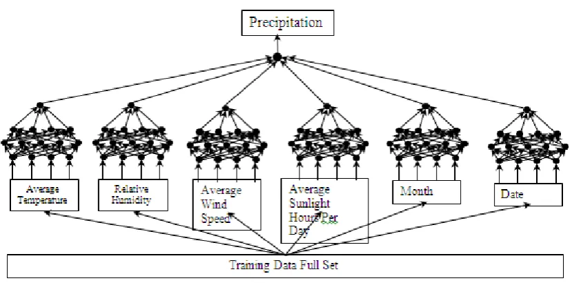
[image:3.595.90.505.523.728.2]Fig. 3 shows the Ensemble Neural Network based on variable Inputs with no hidden layers. The outputs sub-networks for each variable is input to perceptron. Based on the estimates given the all the variable sub networks, the final out put is estimated.
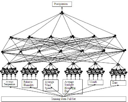
Fig. 4 shows the Ensemble Neural Network based on variable Inputs with hidden Layers. The outputs sub-networks for each variable is input to a set of neurons of the hidden layers whose
out is final fed to perceptron. Based on the estimates given the all the variable sub networks and hidden layers, the final output is estimated.
Figure 4: Ensemble Neural Network based on Variable Inputs with Hidden Layers (ANN-V-M)
Fig. 5 shows the Ensemble Neural Network based on time Inputs with hidden layers. The monthly data of all the variable are fed to the input of each sub network. There will 12 subnetworks in the model to input the data of all the variable for 12 months. The outputs sub-networks for each variable is
Figure 5: Ensemble Neural Network based on Time Inputs with Hidden Layers (ANN-T-M)
4.
SIMULATION
RESULTS
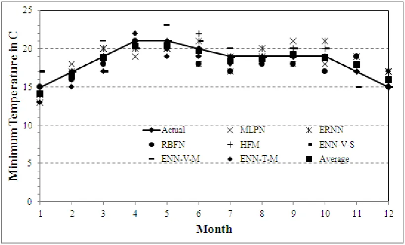
In this section complete set of results obtained from the simulations using MATLAB code and comparisons with the actual data are presented and discussed in detail. Fig. 6 shows the average minimum temperature data for Bangalore for the year of 2010. The values printed in the plot are the actual data physically collected using the rain gauges. In order to predict
the average rainfall for the year 2010, seven neural network models are developed, they are all based on ENNs. Comparisons are made to test the performance of the ANNs developed. Three years of data collected on daily basis is input to the models for training purpose. The training data typically included temperature, humidity and the actual rainfall.
[image:5.595.91.502.503.751.2]Fig 7 shows the comparison among the ENNs predicted maximum temperature values with respect to the actual data. Graphically, the rainfall predicted by the ENN-Average shows better accuracy compared to the SNN. The reason for this
kind of behavior by ENN-Average is the average of all the ENNs used and it gives the best prediction compared to individual ENNs.
Figure 7:Maximum Temperature predicted by the neural networks
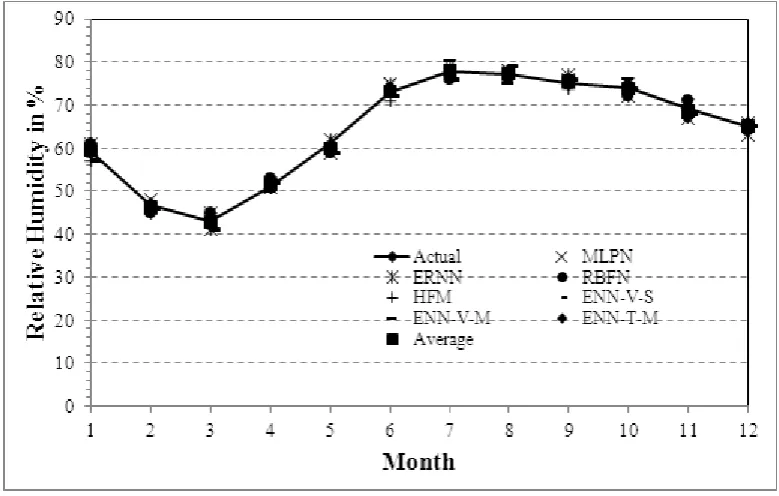
Fig 8 shows the comparison among the ENNs predicted relative humidity values with respect to the actual data. Again, the rainfall predicted by the ENN-Average shows better accuracy compared to the SNN. The reason for this kind of
behavior by ENN-Average is the average of all the ENNs used and it gives the best prediction compared to individual ENNs.
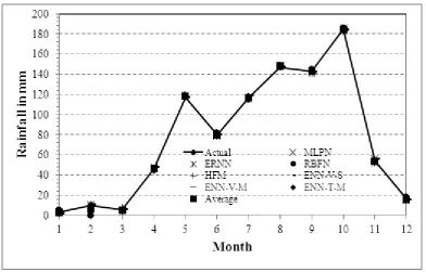
[image:6.595.104.492.119.370.2] [image:6.595.102.492.448.696.2]Figure 9: Average rainfall predicted by the neural networks
Fig 9 shows the comparison among the ENNs predicted rainfall values with respect to the actual data. Again, the rainfall predicted by the ENN-Average shows better accuracy compared to the SNN. The reason for this kind of behavior by ENN-Average is the average of all the ENNs used and it gives the best prediction compared to individual ENNs.
5.
CONCLUSION
In this work, seven Ensemble Artificial Neural Network (ANN) models, namely, Multilayer Perceptron Network (MLPN), Elman Recurrent Neural Network (ERNN), Radial Basis Function Network (RBFN), Hopfield Model (HFM), Ensemble Neural Network based on Variable Inputs with No Hidden Layers (ENN-V-S), Ensemble Neural Network based on Variable Inputs with Hidden Layers (ENN-V-M), Ensemble Neural Network based on Time Inputs with No Hidden Layers (ENN-T-M), are developed to predict the rainfall for one of the large cities of India i.e. Bangalore. Different network models were developed to match the predicted results with the actual data and ENN-Average is found to be the best among all. ENN Average is the average of output of all the ENNs. In order to test this, actual rainfall data was collected in Bangalore city for the calendar years 2007, 2008 and 2009. This data was used as training data for the ANNs and predictions were made for the year 2010. Again these predictions were compared with the actual data to verify the performance of the ANNs. In this study, it has been proved that ENN-Average model based on back propagation algorithm provide better accurate predictions than the SNN and ENN models based on other algorithms. More research need to be carried out in order to improve these models based on ANNs for improving the output for different training algorithms.
6.
REFERENCES
[1] ASCE., 1996. Hydrology Handbook, second edition, American Society of Civil Engineers ASCE, New York.
[2] ASCE., 2001a. Task Committee on Artificial Neural Networks in Hydrology, Artificial Neural Networks in Hydrology. I. Preliminary concepts, Journal of Hydrologic Engineering, ASCE, 52, 115-123.
[3] ASCE 2001b. Task Committee on Artificial Neural Networks in Hydrology, Artificial Neural Networks in Hydrology. II Hydrologic Applications, Journal of Hydrologic Engineering, ASCE, 52, 124-137.
[4] Ashraf, M., Loftis J. C. and Hubbard K.G., 1997. Application of Geostatisticals to Evaluate Partial Weather Station Network. Agricultural Forest Meteorology, 84: 255-271.
[5] Boots, B. N., 1986. Voronoi Thiessen Polygons, Concepts and Techniques in Modern Geography, No. 45, Geo Book, Norwich.
[6] Bras, R.L., and I. Rodriguez-Iturbe. 1985. Random Functions and Hydrology. Addison-Wesley Publishing Company, Reading Massachusetts.
[7] Bras R.L., and R. Colon. 1978. Time Averaged Areal Mean of Precipitation: Estimation and Network Design. Water Resources Research. 14(5):878-888.
[9] Daly, C., R. P. Neilson and D. L. Phillips., 1994. A Statistical Topographic Model for Mapping Climatological Precipitation over Mountainous Terrain. Journal of Applied Meteorology, 33: 140-158.
[10]Deutsch, C. V. and A. G. Journel., 1992. Geostatistical Software Library and User’s Guide, Oxford University Press, New York.
[11]Dingman, S. L., 2002. Physical Hydrology, Prentice Hall, NJ. Freeman, J. A. and Skapura, D. M., 1991. Neural Networks: Algorithms, Applications and Programming Techniques, Addison-Wesley Inc., USA, 1991.
[12]French, M. N., Krajewski, W.F., and Cuykendal, R.R., 1992. Rainfall Forecasting in Space and Time using a Neural Network, Journal of Hydrology, 137, 1-37.
[13]Goodchild, M. F., 1986. Spatial Autocorrelation, Concepts and Techniques in Modern Geography, Geo Books, Norwich
[14]Govindaraju, R. S., and A. R. Rao., 2000. Neural Networks in Hydrology, Kluwer Academic Publishers, Netherlands.
[15]Grayson, R. and B. Gunter, 2001. Spatial Patterns in Catchment Hydrology: Observations and Modeling, Cambridge University Press.
[16]Griffith, D. A., 1987. Spatial Autocorrelation: A Primer, Association of American Geographers, Washington, D. C.
[17]Haan, C. 1977. Statistical Methods in Hydrology. Iowa State University Press, Ames, Iowa.
[18]Haykin, S. 1994. Neural Networks: A Comprehensive Foundation, Macmillan Publishing, NY.
[19]Hodgson, M. E., 1989. Searching Methods for Rapid Grid Interpolation, Professional Geographer, 411: 51-61.
[20]Isaaks, H . E., and R. M. Srivastava., 1989. An Introduction to Applied Geostatisitics, Oxford University Press, New York
[21]Journel, A. G. and C. J. Huijbregts, 1978. Mining Geostatistics, Academic Press, New York.
[22]Krajewski, W. F., 1987. Co-kriging of Radar and Rain Gage Data, Journal of Geophysics Research, 92D8, 9571-9580.
[23]Larson, L. W., and E. L. Peck., 1974. Accuracy of Precipitation Measurements for Hydrologic Forecasting, Water Resources Research, 156, 1687 - 1696.
[24]Maier, H. R., and G. C. Dandy, 1998. The Effect of Internal Parameters and Geometry on the Performance of Back-Propagation Neural Networks: An Empirical Study. Environmental Modeling and Software. 13(2), 193-209.
[25] McCuen, R. H., 1998. Hydrologic Analysis and Design, Prentice-Hall, NJ Navone, H. D., and Ceccatto, H.A., 1994. Predicting Indian Monsoon Rainfall: A Neural Network Approach, Climate Dynamics, 10, 305-312.
[26] Osborn, H. B., K.G. Renard, and J. R. Simanton., 1979. Dense Networks to Measure Convective Rainfall in the Southwestern United States, Water Resources Research, 156 : 1701-1709.
[27] Rodriguez-Iturbe, I. and J.M. Mejia. 1974. The Design of Rainfall Network in Time and Space. Water Resources Research. 10(4):713-728.
[28] Rumelhart, D.E., and J. L. Mclelland, 1986. Parallel Distributed Processing , MIT press, Cambridge, MA.
[29] Salas, J. D.-J., 1993. Analysis and Modeling of Hydrological Time Series, Handbook of Hydrology, D. R. Maidment, ed, Mc-Graw-Hill, NY
[30] Seo, D.-J., Krajewski, W.F., Bowles, D.S. 1990a. Stochastic Interpolation of Rainfall Data from Rain Gages and Radar Using Cokriging - 1. Design of Experiments. Water Resources Research, 26(3), 469-477.
[31] Seo, D.-J., Krajewski, W.F., Bowles, D.S. 1990b. Stochastic Interpolation of Rainfall Data from Rain Gages and Radar Using Cokriging - 2. Results. Water Resources Research, 26(5), 915-924.
[32] Seo, D.-J. and J. A. Smith, 1993. Rainfall Estimation Using Rain gages and Radar: A Bayesian Approach, Journal of Stochastic Hydrology and Hydraulics, 5(1), 1-14.
[33] Seo, D.-J. 1996. Nonlinear Estimation of Spatial Distribution of Rainfall - An Indicator Cokriging Approach. Stochastic Hydrology and Hydraulics, 10,127-150.
[34] Seo, D. J., 1998. Real-time Estimation of Rainfall Fields Using Radar Rainfall and Rain Gage Data, Journal of Hydrology, 208: 37-52.
[35] Simanton, J. R., and H. B. Osborn, 1980. Reciprocal-Distance Estimate of Point Rainfall, Journal of Hydraulic Engineering Division, 106HY7
[36] Singh, V. P., and K. Chowdhury., 1986. Comparing Some Methods of Estimating Mean Areal Rainfall, Water Resources Bulletin, 222, 275-282.
[37] Shepard, D., 1968. A Two-dimensional Interpolation Function for Irregularly Spaced Data, Proceedings of the Twenty-Third National Conference of the Association for Computing Machinery, 517-524.
[38] Smith, J. A., 1993. Precipitation, chapter 3, Handbook of Hydrology, D. R. Maidment ed.. McGraw Hill, New York.
[40]Tabios, G. Q., III and J. D. Salas., 1985. A Comparative Analysis of Techniques for Spatial Interpolation of Precipitation, Water Resources Bulletin, 21: 365-380.
[41]Teegavarapu, R.S.V. and V. Chandramouli., 2005. Improved Weighting Methods, Deterministic and Stochastic Data-Driven Models for Estimation of Missing Precipitation Records, Journal of Hydrology, 312, 191-206.
[42]Teegavarapu, R.S.V. 2006. Use of Universal Function Approximation in Variance-Dependent Surface Interpolation Method: An Application in Hydrology, Journal of Hydrology,
[43]Tobler, W. R., 1970. A Computer Movie Simulating Urban Growth in the Detroit Region. Economic Geography, 46: 234-240.
[44]Tung, Y. K., 1983. Point Rainfall Estimation for a Mountainous Region, Journal of Hydraulic Engineering, American Society of Civil Engineering ASCE, 10910:1386 -1,393.
[45] Vasiliev, I. R., 1996. Visualization of Spatial Dependence: An Elementary View of Spatial Autocorrelation, in Practical Handbook of Spatial Statistics, CRC Press, Boca Raton.
[46] Vieux, B. E., 2001. Distributed Hydrologic Modeling using GIS, Water Science and Technology Library, Kluwer Academic Publishers.
[47] Webster, R. A., and M. A. Oliver., 2001. Geostatistics for Environmental Scientists, John Wiley and Sons, Chichester, UK.
[48] Wei, T. C., and J. L. McGuinness., 1973. Reciprocal Distance Squared Method, a Computer Technique for Estimating Area Precipitation, Technical Report ARS-Nc-8., U.S. Agricultural Research Service, North Central Region, Ohio.