Munich Personal RePEc Archive
Monetary Policy Shocks in a Small Open
Economy: Assessing the ’Puzzles’ of
Monetary Policy by SVAR
Ajluni, Jarir
May 2005
Online at
https://mpra.ub.uni-muenchen.de/22880/
!
& !' () *' (!
!
"
!
# "
$ # "
%&' $
((
& '+ ' + +,
+-! )*+," )*-,"
(
./01
1
/
! %&' 2 $
)**) 3
)**4 )**4 &
%&' %&'
%&'
.
.
1 / 5 )**+
6 7 8 7 )**+
9/ .
7 8 7 )**:
9/ 3- 7 8
7 )**: 9/
; )*-+
9 . < 9.<
'=6 9/
9/ 8 '
)**-6 0
%&'
09/
.
# " 7
#< (( "
/
)**4
8
& *./ ( !) !) 0+( +' * (' , ' (! (1 '0+ 2()+
& 0+ ' *' , +- (!+' " 3( *" !42 44 (! +*0 ! 424
! $ 2
= <
> )
/ + 5 4' ' (! (1 '0+ 2 ' 6*0 !!+ 2(!+' " 3( *" ' !42 44 (! 2+*0 ! 424
!
Central Bank Interest Rate
R
expectations
Market Interest Rates Rm
Broad Money
M
Lending
Consumption
Asset Prices (real estates)
Exchange rate
e
Capital Inflows
Inflation Expectations
Exogenous / Global Shocks
Investment
Aggregate Demand C+I+G+(X-M)
Net Exports
Import prices
Output
Y
Inflation P
Domestic Inflation
Stage I
Stage II
Stage III
!
0
6 . $
? 0
0 0 0
6
?
6 =
& 0+ .+ " +) *+)61( 2 +11+*'4 (1 2(!+' " (!' *' (!
@ 0
%&'
"
0
?
? ?
37
! 2
8 ' 4,,,
; )*-+
& *(!(2+' * ( 2 ' (! 2()+ !/ '0+ 0( ' ! )+!' 1 * ' (! *0+2+
. 8 ' )**- 4,,, 3
4,,A
6 )**B
/ %&'
# " .
=
6 =
3- 9/ C $
3-& 43+* 1 * ' (! !) )+!' 1 * ' (!
! %&'
=
− +
Α =
p
i
t i t i
t Y
Y
1
υ
@ Yt y p m r
*
y p* m* r*
Θ 6 .
3- Θ
9/ D
3-s @?E 9/ D
! %&' / %&' /%&' β , 0 A i A /%&' = − + + Α = Α p i t i t i
t Y t
Y
1
0 δ βυ
! Ai
= Α0 1 0 1 0 0 1 0 0 0 1 0 0 0 0 1 0 0 0 0 1 0 0 0 0 0 0 0 0 1 0 0 0 0 0 0 0 0 1 0 0 0 0 0 0 0 0 1 0 0 0 0 0 0 0 0 0 1 109 108 107 106 105 104 103 102 101 98 97 96 95 94 93 92 91 87 86 85 84 83 82 81 76 75 74 73 72 71 65 64 63 62 61 510 54 51 43 42 32 31 21 α α α α α α α α α α α α α α α α α α α α α α α α α α α α α α α α α α α α α α α α α α α = s r m p y r m p y poil Y * * * * ! %&' %&'
/ /%&' /%&'
< < %&' <F), %&' n
n n n× )−
( n×n & 0
%&' *, ),, 0
! Α0
"
3- .
/ ?
3- $
(
3-C .
C C
!
' 0
. 6 /
(
0
$ .
%&'
& (!4' *' (! (1 1( + /! 7 ' 4+ +4
!
= ∗
= N
i i itY
Y
1 ω
= ∗
= N
i i itP
P
1 ω
= ∗
= N
i
i itM
M
1 ω
= ∗
= N
i i itr
r
1 ω
@ Y* P* M* r*
6 .
i N
3- 9/ 9 6 > 3 . C
# "
G
3-=
+ +
= W
i
it it
it it t
IM EX
IM EX
1 ω
@ EXi ω
7 H . @ tF)*B, )*B:
)**, )**:
@ :
! 4 3- !
"
!
)*B, )*B: )**, 8 )**:
. ! / I &
)*B,
)*B, 0
9
3-3- (
9/ C
" $ > 9/
7
8 ' )**-
& 23 * +4 '4
& "3('0+4 4 '+4' !/ !) / ( )+ 4+ +*' (! (1 '0+ ! +4' *'+)
; %&'
?1/ %&'
?1/
%&'
0
0 1 1 /
+ /=6
%&'
J J
F &.6 /=6 GK.6
[image:11.612.82.533.256.362.2]><7 1' ! )
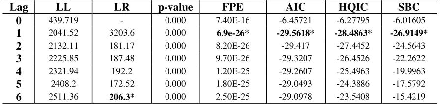
Table 1: Lag order Selection Criterions for the unrestricted VAR
*Bold values Indicates the lag length selection decision for the specified criterion * Degrees of Freedom = 100.
& 23 4+ +43(!4+ !*' (!4 1 (2
! . ' .'>
(
.'>
.'>
.'>
$
.'>
= .'> ? .'> A,
Lag LL LR p-value FPE AIC HQIC SBC
0 439.719 - 0.000 7.40E-16 -6.45721 -6.27795 -6.01605
1 2041.52 3203.6 0.000 6.9e-26* -29.5618* -28.4863* -26.9149*
2 2132.11 181.17 0.000 8.20E-26 -29.417 -27.4452 -24.5643
3 2225.85 187.48 0.000 9.70E-26 -29.3207 -26.4526 -22.2622
4 2321.94 192.2 0.000 1.20E-25 -29.2607 -25.4963 -19.9963
5 2408.2 172.52 0.000 1.80E-25 -29.0493 -24.3886 -17.5792
6 2511.36 206.3* 0.000 2.50E-25 -29.0978 -23.5408 -15.4219
LL: the Log Likelihood statistic. LR: Likelihood Ratio statistics.
FPE: Final Prediction Error. HQI: Hannan and Quinn Information Criterion.
& 6 7(2+4' * (!+' " 0(*. +11+*'4
7 L< (( M
((
(( .'>
A0J
((
. ((
/ + # 23 *' (! '0+ ! !* "4'+2 (1 ! !+83+*'+) 0(*. ! '0+ !'+ +4' '+
! # "
), 4, :
# "
-.02 -.01 0 .01
0 10 20 30
step
95% CI for irf 95% CI for oirf impulse response function (irf) orthogonalized irf
IRF1: r -> e
-.01 0 .01
0 10 20 30
step
95% CI for irf 95% CI for oirf impulse response function (irf) orthogonalized irf
IRF1: r -> y_sa
-.01 0 .01 .02
0 10 20 30
step
95% CI for irf 95% CI for oirf impulse response function (irf) orthogonalized irf
IRF: r -> m
-.01 0 .01 .02
0 10 20 30
step
95% CI for irf 95% CI for oirf impulse response function (irf) orthogonalized irf
! # "
0 ),
$
3 .'>
& 6 ( + /! (!+' " 0(*. +11+*'4
?
? = 0 0
/ + 9 23 *' (! '0+ ! !* "4'+2 (1 ! !+83+*'+) 0(*. ! 0+ -+ /0'+) ,+ /+ : !'+ +4' '+4
< -.05
0 .05 .1
0 10 20 30
step
95% CI for irf 95% CI for oirf impulse response function (irf) orthogonalized irf
IRF: r_G7 -> e
-.04 -.02 0 .02 .04
0 10 20 30
step
95% CI for irf 95% CI for oirf impulse response function (irf) orthogonalized irf
IRF: r_G7 -> y_sa
-.1 -.05 0 .05
0 10 20 30
step
95% CI for irf 95% CI for oirf impulse response function (irf) orthogonalized irf
IRF: r_G7 -> p
-.1 -.05 0 .05
0 10 20 30
step
95% CI for irf 95% CI for oirf impulse response function (irf) orthogonalized irf
!
3-& (!* ) !/ +2 .4
? ((
6<.
(( 6 7 8 7
)**+ . %&'
%&' ((
%&' %&'
$
0
E 8 < )*B4
! 2
%&' ; 0>
0
.
NN
? (( 1 < (( ((
3-?
+1+ +!*+4
[1] Dornbusch, Rudiger (1976), “Expectations and Exchange Rate Dynamics”, Journal of Political Economy, 84(6), p. 1161-76.
[2] Eichenbaum, M and C.L. Evans (1995), “Some Empirical Evidence on the Effects of Shocks to Monetary Policy on Exchange Rates,” Quarterly Journal of Economics, 110, pp. 975-1009 rd. Amsterdam: North-Holland, Elsevier.
[3] Gali, J, (1992), “How well Does the IS-LM Model Fits the Post-war US Data”, Quarterly journal of Economics, 107, 709-738.
[4] Garratt, A. Lee, K. Pesaran, H and Shin, Y, (2002), “A Structural Macroeconomic Model of the UK”, Book under preparation.
[5] ---,(2003),“A long Run Structural Macroeconometric Model of the UK”, Economic Journal, 113, 412-455.
[6] Kim, S. and Roubini, N, (2000), “Liquidity and Exchange Rates in the G7 Countries: Evidence from Identified Vars”, mimeo
[7] Kim, S. and Roubini, N, (2000), “Exchange Rate Anomalies in the Industrial Countries: A Solution with a Structural VAR Approach”, Journal of Monetary Economics, 45, pp.561-586.
[8] Lippi, M and Reichlin, L, (1993), “Dynamic Effects of Aggregate Demand and Supply Disturbances: comment” American Economic Review, 83, 644-652.
[9] Mellander, E. Verdin, A and Warne, A (1992) “Stochastic Trends and Economic Fluctuations in a small open Economy”, Journal of Applied Econometrics, 7, 369-394.