Analyzing Probability Vectors for Named Entity Statistical Machine Transliteration

Analyzing Probability Vectors for Named Entity

Statistical Machine Transliteration

M L Dhore

BRACT’s Vishwakarma Institute of Technology, Pune

S K Dixit

Walchand Institute of Technology, Solapur, India

T D Sonwalkar

BRACT’s Vishwakarma Institute of Technology, Pune

ABSTRACT

Machine transliteration systems are classified as either Rule-based methods or statistical methods. A rule-Rule-based method focuses on transliterating names using lots of human-made rules set. These systems are simple to implement but require huge amount of language expertise. In statistical methods, the importance is given in converting transliteration problem into a classification problem and employs a statistical model to solve this classification problem. Though these methods don’t require expert knowledge of Language model, they need large amounts of bilingual data and good algorithm for training. Currently, basic Markov Chain Model (MM), Extended Markov Chain (EMC), Hidden Markov Model (HMM), Conditional Random Fields (CRF), Decision Tree (DT), Maximum Entropy Markov Model (MEMM) and Support Vector Machine (SVM) are the popular statistical approaches used by many researchers across the globe. This paper focuses on mathematical analysis of different statistical approaches used in machine transliteration of named entity which would be beneficial for many upcoming researchers to know the mathematics used behind the curtains.

General Terms

Keywords

Conditional Random Fields, Decision Trees, Hidden Markov Model, Markov Chain, Statistical Machine Transliteration.

1.

INTRODUCTION

Machine learning is a branch of computer science that deals with the various algorithms that allow a machine to generate patterns based on basic information known as empirical data. In this approach, the basic information is used to capture characteristics of interest for this information based on its underlying probability distribution. This basic data can be seen as examples which show relations between different observed variants. The most important aspect of machine learning is to automatically learn to recognize complex patterns and make intelligent decisions based on this basic information available. The problem is that the set of all possible behaviors when all possible inputs are considered is very large to be covered by a limited set of observed examples. To solve this problem basic data used as examples need to be generalized so that it covers more number of possibilities in less number of examples [1].

Machine Transliteration uses a combination of stochastic, probabilistic and statistical methods to solve various issues related to transliteration problem. For example, increase in length of word makes it highly ambiguous when processed with proper rule-based methods, yielding thousands or millions of possible outcomes. Methods for treating such high number of possible outcomes often involve the use of corpora and Markov models. Statistical Machine transliteration

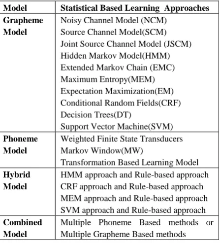
comprises of all quantitative approaches like probabilistic modeling, information theory, and linear algebra. The technology for statistical Machine Transliteration comes mainly from machine learning and data mining, both of which are fields of artificial intelligence that involve learning from data [2]. Table 1 shows the classification of models used in machine transliteration [3].

Table 1. Machine Transliteration Classification

Model Statistical Based Learning Approaches Grapheme

Model

Noisy Channel Model (NCM) Source Channel Model(SCM) Joint Source Channel Model (JSCM) Hidden Markov Model(HMM) Extended Markov Chain (EMC) Maximum Entropy(MEM) Expectation Maximization(EM) Conditional Random Fields(CRF) Decision Trees(DT)

Support Vector Machine(SVM) Phoneme

Model

Weighted Finite State Transducers Markov Window(MW)

Transformation Based Learning Model Hybrid

Model

HMM approach and Rule-based approach CRF approach and Rule-based approach MEM approach and Rule-based approach SVM approach and Rule-based approach Combined

Model

Multiple Phoneme Based methods or Multiple Grapheme Based methods

It has been observed that statistical approaches to transliteration are most popular [4]. One of these approaches is phrase-based statistical machine transliteration and the other is CRF. Statistical approaches are preferred by the researchers due to the many benefits offered by them. Table 2 shows the pros and cons of rule based approaches.

Table 2. Pros and cons of Rule-based Approaches

Advantages Disadvantages  Easy to implement

using handcrafted rules

 Can give better result than statistical methods by enriching language specific rules  Provide good

performance at a relatively high system engineering cost.

 Huge experience and grammatical knowledge of particular language is required

Table 3 shows the pros and cons of statistical approaches. Table 3. Pros and cons of Statistical Approaches

Advantages Disadvantages  It is trainable

 It is adaptable  It is scalable  Low maintenance  Language

independent

 Sufficient training data is required to achieve good result

 Corpora are not available for most of the languages  For better accuracy local

context is required It is also noted that combination of several different models proves to be very successful. Statistical approaches are found to be very effective with grapheme-based model [4]. The combination of grapheme model with statistical approach offers the following benefits.

 Less number of steps required  Less error propagation

 Fewer linguistic resources required

 Performs better than or at par with phoneme-based approaches

 Language independent

 Well suited for statistical probability

2.

RELATED WORK

In 1989, Rabiner reviewed the theoretical aspects of Hidden Markov Modeling and applied it to the selected problems in machine recognition of speech [5]. In the year 1996, Berger presented a maximum-likelihood approach for automatically constructing maximum entropy models and described how to implement this approach efficiently [6]. Conditionally-trained exponential models have been used successfully in many natural language tasks by Nigam in 1999, including document classification [7], sequence segmentation by Beeferman [8] and sequence tagging in 1996 by Ratnaparkhi [9], in 2000 by McCallum [10] and in 2001 by Punyakanok [11]. The best known method for feature induction on exponential models is presented by Della Pietra in 1997[12]. In 2001, Lafferty presented conditional random fields (CRF), a framework for building probabilistic models to segment and label sequence data [13]. In 2004, Altun presented Gaussian process classification for segmenting, a generalization of Gaussian process classification to label sequence learning problem [14]. In 2004, Blunsom described the solution to solve the problems of Viterbi underflow and forward algorithm underflow [15]. In 2006, Oh presented a comparison of different machine transliteration models and showed that the hybrid and correspondence-based models are the most effective [16]. In 2009, Knight wrote a tutorial workbook for natural language researchers and explained the use of expectation-maximization (EM) model with many examples [17]. In the same year, Knight wrote another article describing how to train arbitrary cascades of finite-state machines on end-to-end data [18].

3.

ANYLYSIS OF DECISION TREES

As far as statistical approach for transliteration is considered, transliteration is viewed as assigning label sequences to a set of observation sequences. Label sequence is nothing but transliteration units in target language whereas observation sequence is transliteration units in source language. Generally, supervised machine learning methods are used along with statistical methods for transliteration with the exception of

examples like Maximum Likelihood training with random start.

Analysis of working of four statistical methods is presented in this paper with a common example. Suppose two locations named entities in Devanagari language / / and / / are to be trained which have their English equivalents as /Rampur/ and /Lavanvadi/. These names are syllabified as follows.

ra m

pu r and

la va

n current observation

va

di

In decision tree approach a tree like model of decisions is used along with their possible outcomes. These possible outcomes could be chance event outcomes, resource costs, and utility. It is a method to depict an algorithm in which decision tree is used in decision analysis that is to identify a mechanism which is most likely to reach a goal. Decision tree should be used along with probability models where decisions are to be taken runtime with no recall under incomplete knowledge. Decision tree is used to describe calculations of conditional probabilities [19].

Classification using decision tree approach yields the output as a binary tree like structure called a decision tree, where each branch node represents a choice between a number of possibilities, and each leaf node represents a classification or decision. A decision tree model contains rules to predict the target variable.

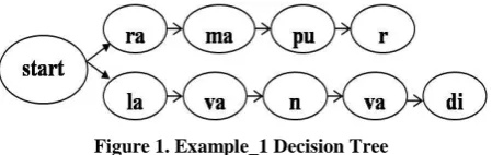
For constructing a decision tree, a set of nodes equal to number of distinct output tags is taken along with a special start node. For each input in the training example, an edge is added to the tree from previous output tag to the current output tag. Initially, edge is added from start node to first output tag as shown in figure 1

.

Figure 1. Example_1 Decision Tree

Figure 2. Example_2 Decision Tree

4.

ANALYSIS MARKOV MODEL AND

EXTENDED MARKOV CHAIN

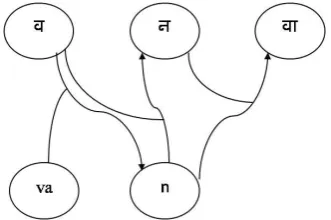
The simplest Markov model is the Markov chain. It models the state of a system with a random variable that changes through time. In simple MM, the Markov property suggests that the distribution for this variable depends only on the distribution of the previous state. Various kinds of information sources are involved in the transliteration problem. It is not possible to represent this information using conventional MM. So, extended Markov chain is used to represent transliteration problem [20]. This can be explained using same example used above. Figure 3 shows an example of extended Markov chain formation.

Figure 3. Example of Extended Markov Chain

Source language Units are { , , , , } and target language units are { la,va,n,va,di }.

Simple Markov window can be demonstrated as follow.

la va n va di

Extended Markov window can be demonstrated as follow

la va n va di

Suppose that source word S is segmented into a sequence of syllabified units S1, S2, …Sn where Si is a source language

unit. Similarly Ti is a target language unit. Let us say P(S, T)

is the probability that a Source word S is transliterated to a target word T. Finding K such that P(S, K) is maximized when T is given. The value P (K|T) can be calculated using the following equation which follows Extended Markov property,

Decision making in Extended Markov chain is done based on the probability model generated after applying proper probability distribution methods. Probability model is represented using a probability vector generated after using probability distribution formula for each input given in the training example. This method of generating probability model is true for rest of the two methods, namely Hidden Markov model and Conditional Random fields. Only the formula used to calculate probability distribution is different. These probabilities are calculated based on values of feature functions.

Feature function in the context of transliteration can be defined for each transliteration unit (TU) in training example as,

, if source-target language TU pair exist = 0, otherwise.

where STU is Source language transliteration unit and TTU is target language transliteration unit.

For example, for pair न n,

f (n , न) = 1

f (la ,न) =0 and so on.

Probability distribution of EM chain can be given as

where si is source language TU and is target language TU.

Therefore, probability vector can be calculated by calculating individual probabilities as follow

For pair न n,

f(n, )=1, f(n, ) =0 and f(n, ) =0

P(n, )

=

P(n, )

=

= 0.5761

P(n, ) =

P(n, ) =

= 0.2194

P(n, ) =

P(n, ) =

In this way, probability vector is generated which is also known as probability model for given set of inputs is shown in table 4.

Table 4. Probability Vector of EM Chain

ra 0.5761 0.2194 0.3333 0.3333 0.3333 0.3333 0.3333 0.3333 0.2194 m 0.2194 0.5761 0.2194 0.3333 0.3333 0.3333 0.3333 0.3333 0.3333 pu 0.3333 0.2194 0.5761 0.2194 0.3333 0.3333 0.3333 0.3333 0.3333 r 0.3333 0.3333 0.2194 0.5761 0.2194 0.3333 0.3333 0.3333 0.3333 la 0.3333 0.3333 0.3333 0.2194 0.5761 0.2194 0.3333 0.3333 0.3333 va 0.3333 0.3333 0.3333 0.3333 0.2194 0.5761 0.2194 0.3333 0.3333 n 0.3333 0.3333 0.3333 0.3333 0.3333 0.2194 0.5761 0.2194 0.3333 va 0.3333 0.3333 0.3333 0.3333 0.3333 0.3333 0.2194 0.5761 0.2194 di 0.2194 0.3333 0.3333 0.3333 0.3333 0.3333 0.3333 0.2194 0.5761

5.

ANALYSIS OF HMM

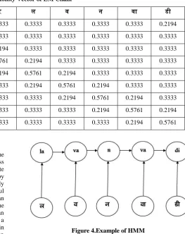
A hidden Markov model is a statistical model in which the system being modeled is supposed to be a Markov process with unobserved states. Hidden Markov model is a finite-state automaton where transition between states is given by probability functions. In Markov model, the state is directly visible to the observer. Hidden Markov model is very useful to simulate processes that are generally unknown but that can be observed through a sequence of symbols. For example, the sequence of letters that forms a word in a given language can be considered as a sequence of symbols given as output by a Hidden Markov model. The Hidden Markov model starts in an initial state and performs a sequence of transitions between states by giving a new letter as output at each transition until it stops at a final state. Generally, several state sequences or state paths can correspond to a single word. It is possible to compute the probability of each path and therefore compute the most probable path corresponding to a word. This is called decoding, for which an efficient decoding algorithm like Viterbi decoding algorithm is used. In a hidden Markov model, the state is not directly visible, but output which is dependent on the state is visible. Each state has a probability distribution over the possible output tokens. Hence, the sequence of tokens generated by a hidden Markov model gives some information about the sequence of states. In Hidden Markov model, probability of the output tag depends on current input tag and previous output. For our common example, source language units are { , , , , } and target language units are { la,va,n,va,di} then the Hidden Markov model window can be demonstrated as shown below.

la va n va di

Suppose that source word S is segmented into a sequence of syllabified units as , , … where is a source language unit. Similarly, is a target language unit.

Figure 4.Example of HMM

In HMM, probability of output tag given an input sequence can be given by following formula [21],

∑

∑

The probability distribution of HMM is calculated below using Kupeic’s method.

For the same pair,  n,

f(n, )= 1

So, P (n, )

=

So, P (n, )

=

Table 5. Probability Vector of HMM

ra 0.2466 0.1111 0.1111 0.1111 0.1111 0.1111 0.1111 0.1111 0.1111 m 0.1111 0.2466 0.1111 0.1111 0.1111 0.1111 0.1111 0.1111 0.1111 pu 0.1111 0.1111 0.2466 0.1111 0.1111 0.1111 0.1111 0.1111 0.1111 r 0.1111 0.1111 0.1111 0.2466 0.1111 0.1111 0.1111 0.1111 0.1111 la 0.1111 0.1111 0.1111 0.1111 0.2466 0.1111 0.1111 0.1111 0.1111 va 0.1111 0.1111 0.1111 0.1111 0.1111 0.2466 0.1111 0.1111 0.1111 n 0.1111 0.1111 0.1111 0.1111 0.1111 0.1111 0.2466 0.1111 0.1111 va 0.1111 0.1111 0.1111 0.1111 0.1111 0.1111 0.1111 0.2466 0.1111 di 0.1111 0.1111 0.1111 0.1111 0.1111 0.1111 0.1111 0.1111 0.2466

6.

ANALYSIS OF CRF

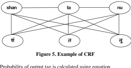
A conditional random field is defined as an undirected graphical model, or Markov random field, globally conditioned on X, the random variable representing observation sequences. Formally, definition of CRF is given as G = (V, E) to be an undirected graph such that there is a node v Є V corresponding to each of the random variables representing an element of Y. If each random variable obeys the Markov property with respect to G, then (Y, X) is a conditional random field. In theory the structure of graph G may be arbitrary, provided it represents the conditional independencies in the label sequences being modeled. The simplest and most common graph structure is that in which the nodes corresponding to elements of Y form a simple first-order chain. Figure 5 is an example of such model.

Figure 5. Example of CRF

Probability of output tag is calculated using equation e p ∑ ∑

where ( , , x, i) is a transition feature function of the entire observation sequence and the labels at positions i and i−1 in the label sequence; ( , x, i) is a state feature function of the label at position i and the observation sequence; and and are parameters to be estimated from training data[22].

Potential Function:

Joint distribution over elements of Y is factorized into a normalized product of strictly positive, real-valued potential functions using graphical structure of CRF. Each potential function manipulates a limited set of the random variables represented by vertices in graph G. This ensures that none of the potential function points to any pair of random variables whose vertices are not directly connected to each other. If any

of the two vertices appear together then this relationship is explicitly mentioned.

Isolated potential functions depict the constraints on the configurations of the random variables on which the function is defined. They don’t have direct probabilistic interpretation which affects the global probability configuration. As a result, a global configuration with a high probability would satisfy more of these constraints as compared to a global configuration with a low probability [22-24].

Following the same analogy followed for above two models, probability distribution of CRF is defined as

∑

f (n, )= 1 f (n, ) =0

P (n, ) =

P (n , ) =

= 0.2536

P (n, ) =

P (n, ) =

= 0.0932

Table 6. Probability Vector of CRF

ra 0.2536 0.0932 0.0932 0.0932 0.0932 0.0932 0.0932 0.0932 0.0932 m 0.0932 0.2536 0.0932 0.0932 0.0932 0.0932 0.0932 0.0932 0.0932 pu 0.0932 0.0932 0.2536 0.0932 0.0932 0.0932 0.0932 0.0932 0.0932 r 0.0932 0.0932 0.0932 0.2536 0.0932 0.0932 0.0932 0.0932 0.0932 la 0.0932 0.0932 0.0932 0.0932 0.2536 0.0932 0.0932 0.0932 0.0932 va 0.0932 0.0932 0.0932 0.0932 0.0932 0.2536 0.0932 0.0932 0.0932 n 0.0932 0.0932 0.0932 0.0932 0.0932 0.0932 0.2536 0.0932 0.0932 va 0.0932 0.0932 0.0932 0.0932 0.0932 0.0932 0.0932 0.2536 0.0932 di 0.0932 0.0932 0.0932 0.0932 0.0932 0.0932 0.0932 0.0932 0.2536

This method avoids label-bias problem. Also, calculation of tag sequence is not independent of tags other than current (as probability distribution is calculated over entire input sequence).

7.

OUTCOME OF ANALYSIS

An efficient statistical transliteration should provide multiple possible solution tags for a given observation so that even if one first output is not correct, one of the subsequent outputs would give correct candidate tag.

Label-bias degrades the accuracy of ranking candidate outputs in sequence labeling.

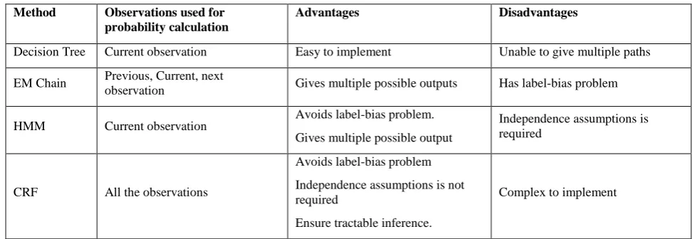
Independence assumption means that the calculation of probability for a tag is independent of all observation except the current tag. It is desirable in many sequence labeling tasks. But for transliteration, probabilities for a particular are taken on the entire observation. So, there is no requirement of independence assumption. It is advantageous to avoid it. Tractable inference is required to predict multiple possible paths starting from a particular tag. This is also important to get multiple candidate output tags for a particular observation. Due to all above reasons, CRF is suitable for machine transliteration. Table 7 shows the analysis of statistical approaches.

Table 7. Analysis of Statistical Approaches

Method Observations used for probability calculation

Advantages Disadvantages

Decision Tree Current observation Easy to implement Unable to give multiple paths

EM Chain Previous, Current, next

observation Gives multiple possible outputs Has label-bias problem

HMM Current observation Avoids label-bias problem. Gives multiple possible output

Independence assumptions is required

CRF All the observations

Avoids label-bias problem Independence assumptions is not required

Ensure tractable inference.

Complex to implement

8.

ACKNOWLEDGMENTS

We express our gratitude to Ashutosh Marathe, Dean QA, Nitin Patki, Dean Examination, Dr. J S Umale, Dr. S T Patil, Priyadharshan Dhabe, S S Pawale, Rajashree Agarwal, P P Ghadekar, R N Patil, N Z Tarapore, G D Bhutkar, Neelam Chandolikar, D P Pawar, Rupali Pawar, Shubhda Deshmukh, Mugdha Shah, Aparna Mete, Ashwini Shingare, D J Joshi, A A Deshpande, Babita Rathod, Sangeeta Wadekar, Saraswati Jadhav, S V Jagtap, Namrata Gawande, V A Godbole, Nachiket Kulkarni and Suresh Nagargoje of Vishwakarma Institute of Technology for their continuous encouragement to carry out the research in the area of Machine Transliteration. We also thank to Balasaheb Lende, Jyoti Dhore, Namrata Gaigol, Mohan Gaigol, Ramdas Gawande, S B Choudhari, Sunil Dhore, Promod Patil, Bhagwan Gawai, Pravin Anjikar,

Sheetal Patil, Anil Mhaske, Anant Wadhokar, Amol Kale for their valuable guidance of Marathi and Hindi linguistics. Special thanks to S R Bandewar who helped in the statistical analysis of machine transliteration.

9.

REFERENCES

[1] Mitchell, T. 1997. Machine Learning, McGraw Hill [2] Christopher D. Manning, Hinrich Schutze. 1999.

Foundations of Statistical Natural Language Processing, MIT Press

[4] Li Haizhou, Kumaran A, Vladimir Pervouchine and Min Zhang, 2009. Report of NEWS Machine Transliteration Shared Task

[5] L. Rabiner. 1989. A tutorial on Hidden Markov Models and selected applications in Speech Recognition. Proceedings of IEEE, Vol 77, No. 2, pp. 257-296 [6] A. L. Berger, S. D. Pietra, and V. J. Della Pietra. 1996. A

maximum entropy approach to natural language processing, Computational Linguistics, vol. 22, no. 1, pp. 39–71

[7] Nigam, K., Lafferty, J., & McCallum, A. 1999. Using maximum entropy for text classification. IJCAI-99 Workshop on Machine Learning for Information Filtering, pp. 61–67

[8] Beeferman, D., Berger, A., & Lafferty, J. D. 1999. Statistical models for text segmentation. Machine Learning, 34, pp. 177–210.

[9] Ratnaparkhi, A. 1996. A maximum entropy model for part-of speech tagging. In E. Brill and K. Church (Eds.), Proceedings of the conference on empirical methods in natural language processing, Somerset, New Jersey: Association for Computational Linguistics, pp. 133–142 [10]McCallum, A., Freitag, D., & Pereira, F. 2000.

Maximum Entropy Markov models for information extraction and segmentation. Proceedings of ICML pp. 591–598

[11]Punyakanok, V., and Roth, D. 2001. The use of classifiers in sequential inference. NIPS 13.

[12]Della Pietra, S., Della Pietra, V. J., & Lafferty, J. D. 1997. Inducing features of random fields. IEEE Transactions on Pattern Analysis and Machine Intelligence, 19, pp. 380–393.

[13]Lafferty, J., McCallum, A., & Pereira, F. 2001. Conditional random fields: Probabilistic models for segmenting and labeling sequence data. Proc. ICML. [14]Yasemin Altun, Thomas Hofmann, and Alexander J.

Smola, 2004. Gaussian Process Classification for Segmenting and Annotating Sequences, Proceedings of the 21 st International Conference on Machine Learning, Canada

[15]Phil Blunsom, 2004. Hidden Markov Models

[16]Jong-Hoon Oh, Key-Sun Choi, and Hitoshi Isahara, 2006. A Machine Transliteration Model Based on Correspondence between Graphemes and Phonemes, ACM Transactions on Asian Language Information Processing, Vol. 5, No. 3, pp. 185–208.

[17]Kevin Knight, 2009. Bayesian Inference with Tears, a tutorial workbook for natural language researchers [18] Kevin Knight, 2009. Training Finite-State Transducer

Cascades with Carmel

[19]Y. Yuan and M J Shaw, 1995. Introduction of Fuzzy Decision Trees, Fuzzy sets and Systems, pp 125-139 [20]Sung Young Jung, Sung Lim Hong and Eunok Pack,

2000. An English to Korean transliteration model of Extended Markov Window, Proceeding COLING 2000 Proceedings of the 18th conference on Computational linguistics , Volume 1, pp 383-389.

[21]GuoDong Zhou and Jian Su, 2002. Named Entity Recognition using an HMM-based Chunk Tagger, Proceedings of the 40th Annual Meeting of the Association for Computational Linguistics (ACL), Philadelphia, pp. 473-480.

[22]Hanna M. Wallach, 2004. Conditional Random Fields: An introduction, University of Pennsylvania CIS Technical Report MS-CIS-04-21, pp. 1-9

[23]Charles Sutton and Andrew McCallum, An Introduction to conditional random fields for relational learning, University of Massachusetts, USA

[24]Sunita Sarawagi and WilliamW. Cohen, Semi-Markov Conditional Random Fields for Information Extraction, Indian Institute of Technology Bombay, India

10. AUTHORS PROFILE

M. L. Dhore has completed ME in Computer Science and Engineering from NITR, Chandigarh, Thapar University, Punjab, India in 1998.Currently he is working as Associate Professor in Computer Engineering Department at Vishwakarma Institute of Technology, Pune, Maharashtra, India. Presently he is pursuing his Ph.D. from University of Solapur, Maharashtra, India, in Machine Transliteration. His areas of interest are Webpage Localization and Computer Networking.

Dr. S. K. Dixit has received Ph.D. in Electronics from Shivaji University, Kolhapur, Maharashtra, India, in 2002. Currently he is working as Head and Professor in Department of Electronics and Telecommunication at Walchand College of Engineering, Solapur, Maharashtra, India