A frequency domain test for propriety of complex valued vector time series

Chandna, Swati and Walden, A. (2016) A frequency domain test for

propriety of complex-valued vector time series. IEEE Transactions on Signal

Processing 65 (6), pp. 1425-1436. ISSN 1053-587X.

Downloaded from:

Usage Guidelines:

Please refer to usage guidelines at or alternatively

A Frequency Domain Test for Propriety of

Complex-Valued Vector Time Series

Swati Chandna and A. T. Walden, Senior Member, IEEE

Abstract

This paper proposes a frequency domain approach to test the hypothesis that a stationary

complex-valued vector time series is proper, i.e., for testing whether the vector time series is uncorrelated with its

complex conjugate. If the hypothesis is rejected, frequency bands causing the rejection will be identified

and might usefully be related to known properties of the physical processes. The test needs the associated

spectral matrix which can be estimated by multitaper methods using, say,K tapers. Standard asymptotic distributions for the test statistic are of no use since they would require K → ∞,but, as K increases so does resolution bandwidth which causes spectral blurring. In many analyses K is necessarily kept small, and hence our efforts are directed at practical and accurate methodology for hypothesis testing for

small K. Our generalized likelihood ratio statistic combined with exact cumulant matching gives very accurate rejection percentages. We also prove that the statistic on which the test is based is comprised of

canonical coherencies arising from our complex-valued vector time series. Frequency specific tests are

combined using multiple hypothesis testing to give an overall test. Our methodology is demonstrated on

ocean current data collected at different depths in the Labrador Sea. Overall this work extends results

on propriety testing for complex-valued vectors to the complex-valued vector time series setting.

Index Terms

Generalized likelihood ratio test (GLRT), improper complex time series, multichannel signal, multiple

hypothesis test, spectral analysis.

I. INTRODUCTION

There has long been an interest in time series motions on the complex plane: the rotary analysis method

decomposes such motions into counter-rotating components which have proved particularly useful in the

study of geophysical flows influenced by the rotation of the Earth [11], [12], [23], [37], [38].

Let a complex-valued p-vector-valued discrete time series be denoted{Zt}.This has ast-th element,

(t∈Z),the column vectorZt= [Z1,t, . . . , Zp,t]T.A length-N realization of{Zt}namely z0, . . . ,zN−1

has zt∈Cp.In this paper we assume the p processes are jointly second-order stationary.

We propose a frequency domain approach to testing the hypothesis that a complex-valued p

-vector-valued time series is proper, i.e., for testing whether the vector time series {Zt} is uncorrelated with

its complex conjugate{Z∗_t}.If we denote the covariance sequence between these terms by {rZ,τ} then propriety corresponds torZ,τ =0 for allτ ∈Z,orRZ(f) =0over the Nyquist frequency range, where

RZ(f)is the Fourier transform of{rZ,τ}. Otherwise the time series is said to be improper; the practical importance and occurrence of improper processes is discussed in, e.g., [1], [23], [26], [27] and [32].

In this paper we take as an example a multi-component complex-valued ocean current time series

recorded in the Labrador Sea. Frequency domain analysis is particularly useful in a scientific setting:

if the hypothesis is rejected, frequency bands causing the rejection can be identified and quite possibly

related to known properties of the physical processes.

Analogous tests applicable to complex-valued random vectors — rather than time series — are given

by, e.g., [33] and [39]. However, we must consider new methodology suitable for very limited degrees of

freedom. Our test uses the associated spectral matrix which can be estimated by multitaper methods using,

say,K tapers. Standard asymptotic distributions for the test statistic are useless as they require K→ ∞,

but, as K increases so does resolution bandwidth which causes spectral blurring. In many analyses K

is necessarily kept small, and hence our efforts are directed at practical and accurate methodology for

hypothesis testing for smallK. Our generalized likelihood ratio statistic combined with exact cumulant

matching gives very accurate rejection percentages.

For the scalar case, (p= 1),a parametric hypothesis test for propriety of complex time series is given

in [34], [35]. This is based on the series being well-modelled by a Mat´ern process in [34] or complex

autoregressive process of order one in [35], and utilises the χ2 distribution for the test statistic, an asymptotic result. This is in contrast to our approach which (i) is suitable forp >1,(ii) is nonparametric,

so does not rely on a good fit to a parametric model, and (iii) develops a suitable non-asymptotic

distribution for the test statistic.

Our frequency-specific test statistic is comprised of canonical coherencies arising from the

complex-valued vector time series, analogous to the situation for complex-complex-valued random vectors. Canonical

analysis of real-valued vector time series has been extensively studied and utilised (e.g., [24], [31]),

mostly in the context of parametric autoregressive moving-average (ARMA) models. Miyata [25] looked

at real-valued vector time series, and developed canonical correlations through linear functions of discrete

are sample values, we instead work with the orthogonal processes underlying the complex-valued vector

time series, and whose variances and cross-covariances correspond exactly to the spectral components.

We are thus able to define population — as well as sample — canonical coherencies for complex-valued

vector time series.

We use multiple hypothesis testing to develop an overall —rather than frequency-specific — test of

propriety for the time series. Our methodology is demonstrated on ocean current data collected at different

depths in the Labrador Sea.

At the refereeing stage our attention was drawn to the contemporaneous conference paper [36]. Unlike

[36] the current paper shows that our test statistic — which appeared first in [7, Chapter 5] — is comprised

of canonical coherencies and we give a simple scaled F distribution (obtained via cumulant matching)

for deriving rejection percentages. The way the tests are constructed and used in the two cases are also

different, and this is discussed in Section IX.

A. Contributions

Following some background in Section II on complex-valued time series, and the statistical properties

of their spectral matrix estimators under the Gaussian stationary assumption for{Zt},the contributions

of this paper are as follows:

1) In Section III we formally derive the canonical coherencies for {Zt} and {Z∗t} and show in

Section IV how a test statistic T(f) for testing RZ(f) = 0 arises from the sample canonical

coherencies.

2) After giving further research context in Section V, we carefully study the statistical properties of

M(f) = −2KlogT(f) in Section VI, concentrating on the small K case. We show that Box’s

scaled chi-square approximation is exact forp= 1 but not for p > 1,and we derive the cumulants

ofM(f).

3) In Section VII we show that for p > 1 and small K matching the first three cumulants of M(f)

exactly to a scaledF distribution performs at least as well as competitor methods.

4) A simulation study is given in Section VIII which supports the use of the scaledF approximation

for M(f) for the complex-valued vector time series setting.

5) In Section IX we describe the use of multiple hypothesis tests for developing an overall — rather

than frequency-specific — test of propriety for the time series. Simulations show good behaviour

under both the null hypothesis (Section IX-D) and under alternatives (Section IX-E).

6) A data analysis using vector valued oceanographic time series is given in Section X which shows

bands cause the rejection, which may be linked to the physical processes involved.

II. BACKGROUND

We will first show how propriety is linked to matrices in the frequency domain and then discuss the

estimation of these matrices from complex vector-valued Gaussian stationary time series.

A. Some Definitions

We consider a complex-valued p-vector-valued discrete time stochastic process {Zt} whose tth

el-ement, t ∈ Z, is the column vector Zt = [Z1,t, . . . , Zp,t]T, and without loss of generality take each

component process to have zero mean. The sample interval is ∆t and the Nyquist frequency is f_N =

1/(2∆t). We assume the p processes are jointly second-order stationary (SOS), i.e., the covariance

cov{Zl,t+τ, Zm,t}

def

=E{Zl,t+τZm,t∗ }and the complementary-covarianceccov{Zl,t+τ, Zm,t}

def

=E{Zl,t+τZm,t},

1≤l, m≤p,are functions ofτ only. Note that ccov{Zl,t+τ, Zm,t}= cov{Zl,t+τ, Zm,t∗ },the covariance between one process and the complex conjugate of the other.

A matrix covariance sequence is then given by sZ,τ = E{Zt+τZHt }, τ ∈ Z, where superscript H denotes Hermitian (complex-conjugate) transpose; we define the (l, m)th element as sZ,lm,τ

def

= (sZ,τ)lm. A matrix complementary-covariance follows as rZ,τ = E{Zt+τZTt}, τ ∈ Z, with (l, m)th element rZ,lm,τ

def

= (rZ,τ)lm.From their definitions we see that

sZ,lm,τ =s∗Z,ml,−τ; rZ,lm,τ =rZ,ml,−τ,1≤l, m≤p.

We assume ∑∞_τ=−∞|sZ,lm,τ| < ∞ and

∑_∞

τ=−∞|rZ,lm,τ| < ∞, for 1 ≤ l ≤ m ≤ p, which means that the Fourier transforms SZ,lm(f) and RZ,lm(f) for 1 ≤ l, m ≤ p, exist and are bounded and continuous. For |f| ≤ f_N, the corresponding matrices are SZ(f) = ∆t

∑_∞

τ=−∞sZ,τe−i2πf τ∆t and RZ(f) = ∆t

∑_∞

τ=−∞rZ,τe−i2πf τ∆t,respectively. Then

rZ,τ =rTZ,−τ =⇒ RZ(f) =RTZ(−f). (1)

The covariance stationarity means that there exists an orthogonal process Z(f) such that Zt =

∫1/2

−1/2e

i2πf t_{dZ(f) [41, p. 317] and Z}∗ t =

∫1/2

−1/2e

i2πf t_dZ∗_{(−f),with [38]} E{dZ(f)dZH(f′)}=

    

SZ(f)df, f =f′

0, otherwise,

and

E{dZ(f)dZT(f′)}=     

RZ(f)df, f =−f′

B. Proper Processes

If rZ,τ =0 for allτ ∈Z,orRZ(f) =0 for all|f| ≤f_N,then the process {Zt}is said to be proper. Equivalently we see that if{Zt}is uncorrelated with its complex conjugate{Z∗t},then the vector-valued

process is proper. This paper considers the problem of testing that the vector process is proper. From (1)

we see that if RZ(f) =0 for f >0then it is also 0 forf <0. Hence we need to test:

H0 :RZ(f) =0 for allf ≤f_N. (2)

Remark 1: Based on the naming convention adopted in [32, p. 41] for complex-valued vectors, an

alternative would be to call the component processes ‘jointly proper.’

C. Spectral Matrices

Here we define spectral matrices for both the so-called composite real and augmented complex

representations of the series. Let

Zl,t =Xl,t+ iYl,t, (3)

with {Xl,t} and {Yl,t} real-valued, for l = 1, . . . , p. The composite real representation of the series

is given by Vt = [XTt,YTt]T = [X1,t, . . . , Xp,t, Y1,t, . . . , Yp,t]T, a real 2p-dimensional vector-valued

Gaussian stationary process. If

T def= 

Ip iIp Ip −iIp



, (4)

we see that

T Vt=



Xt+ iYt Xt−iYt

 =

 Zt

Z∗_t



=Ut, (5)

where Ut = [ZTt,ZHt ]T = [Z1,t, . . . , Zp,t, Z1∗,t, . . . , Zp,t∗ ]T is the augmented complex representation of the series, a complex2p-dimensional vector-valued Gaussian stationary process.

The spectral matrix for Vt is given by

SV(f) =



SXX(f) SXY(f)

SY X(f) SY Y(f)



_∈C2p×2p_{. (6)}

The spectral matrix for Ut is SU(f) =T SV(f)TH and has the form

SU(f) =



SZ(f) RZ(f)

RH_Z(f) ST_Z(−f) 

_∈C2p×2p_{. (7)}

The matrixSU(f)can be written in the alternative covariance matrix formE{U(f)UH(f)}=SU(f)df,

where

Remark 2: Consider (7). We see that testing RZ(f) = 0 is the same as testing the independence of

the two complex Gaussianp-vectors,dZ(f)anddZ∗(−f).This simple fact enables us to utilise results

from the propriety testing of complex-valued vectors.

D. Estimation

WithSU(f)in (7) seen to be of central importance we now turn to its estimation and related statistical

properties.

Given a length-N sampleV0, . . . ,VN−1, formhk,tVtusing a suitable set ofK length-N orthonormal data taper sequences {hk,t}, k = 0, . . . , K −1, and compute JV,k(f) = ∆1t/2

∑N−1

t=0 hk,tVte−i2πf t∆t. In this work we use sine tapers (e.g., [40]).

As N → ∞, with the number of degrees of freedom, K fixed, and with the given taper properties,

{JV,k(f), k = 0,1, . . . , K −1} are proper, independent and identically distributed random vectors distributed as

JV,k(f)

d

=N₂C_p(0,SV(f)), 0<|f|< f_N, (9)

for k = 0, . . . , K −1 (e.g., [8]). As JU,k(f) =T JV,k(f), as N → ∞, with K fixed, {JU,k(f), k=

0,1, . . . , K−1}are also a set of proper, independent and identically distributed random vectors each of

which are distributed as

JU,k(f)

d

=NC

2p(0,SU(f)), 0<|f|< f_N. (10)

The probability density function (PDF) of JU,k(f) — a proper Gaussian vector in C2p is given by [29]

π−p[det{SU(f)}]−1exp

{

−JH_U,k(f)S_U−1(f)JU,k(f)

}

. (11)

The independence of JU,k(f)’s allows us to write the joint PDF of JU,0(f), . . . ,JU,K−1(f) as the

product of their marginal densities given by (11). So the likelihood function,gJ(SU(f)|JU,0(f), . . . ,JU,K−1(f)),

ofSU(f) given JU,0(f), . . . ,JU,K−1(f),is given by

[πpdet{SU(f)}]−Kexp

{

−

K∑−1

k=0

JH_U,k(f)S_U−1(f)JU,k(f)

}

. (12)

NowSˆU(f) is the sample covariance matrix of{JU,k(f);k= 0,1, . . . , K−1}, i.e.,

ˆ

SU(f) =

1

K K_∑−1

k=0

JU,k(f)JHU,k(f) =



SˆZ(f) RˆZ(f)

ˆ

RH_Z(f) SˆT_Z(−f) 

. (13)

Noting that the argument ofexp{·}in (12) is scalar, and so is equal to its trace, and recalling the linearity

and cyclicity of the trace operator, we can write

gJ = [πpdet{SU(f)}]−Kexp

{

−Ktr{S−_U1(f) ˆSU(f)}

}

dependence of gJ on its arguments are not shown explicitly.

For a finite value of N, {JU,k(f);k= 0,1, . . . , K−1} are proper random variables with

JU,k(f)

d

=N₂C_p(0,SU(f)), WN <|f|< f_N −WN, (15)

where [−WN, WN]is the extent of the spectral window induced by tapering [8]. For sine tapers

WN = (K+ 1)/[2(N + 1)∆t], (16)

(e.g., [40]). Therefore, in practice, we have to restrict interest to frequencies in the range WN <|f|<

f_N −WN.

III. CANONICALCOHERENCIES

From Remark 2 we know that the structure of the testing problem will be related to measures of

coherence between vector-valued processes, and so we next turn our attention to the idea of canonical

coherence. We start by developing the framework required for complex-valued time series.

Let {ξ_t} be the cross-correlation of complex-valued deterministic matrix sequence {At} with time

series {Zt}:

ξ_t=A∗⋆Zt

def

=

∞

∑

u=−∞

A∗_uZt+u.

Next let{η_t} be the cross-correlation of complex-valued deterministic matrix sequence {Bt} with time

series {Z∗_t}:

η_t=B∗⋆Z∗_t def=

∞

∑

u=−∞

B∗_uZ∗_t+u. Component-wise we have

       

ξ1,t ξ2,t .. . ξp,t         =∑ u        

a∗_11,u . . . . . . a∗_1p,u a∗_21,u . . . . . . a∗_2p,u

..

. ...

a∗_p1,u . . . . . . a∗_pp,u

               

Z1,t+u Z2,t+u

.. .

Zp,t+u

        . (17)

So, for j= 1, . . . , p,

ξj,t =

∑

u

a∗_j1,uZ1,t+u+· · ·+

∑

u

a∗_jp,uZp,t+u. (18)

The spectral representation theorem allows us to writeξj,t, j= 1, . . . , p andZl,t, l= 1, . . . , p, as

ξj,t= ∫ f_N

−f_N

ei2πf t∆t_dZξ

j(f); Zl,t=

∫ f_N

−f_N

ei2πf t∆t_dZl(f).

Substituting the spectral representation for Zl,t in the lth sum on the right of (18), we get

∑

u

a∗_jl,uZl,t+u =

∫ f_N

−f_N

ei2πf t∆t_A∗

whereAjl(f) =

∑

uajl,ue−i2πf u∆t. Proceeding in analogous fashion, and using the fact that the orthog-onal process in a spectral representation is unique [10, p. 34], we obtain

dZξj(f) = A

∗

j1(f)dZ1(f) +. . .+A∗jp(f)dZp(f)

def

= AH_j (f)dZ(f).

So

ξj,t =

∫ f_N

−f_N

ei2πf t∆t_AH

j (f)dZ(f). (19)

For{η_t} a similar procedure gives

dZηj(f) = B

∗

j1(f)dZ1∗(−f) +. . .+Bjp∗ (f)dZp∗(−f)

def

= BH_j (f)dZ∗(−f),

and

ηj,t =

∫ _f

N

−f_N

ei2πf t∆t_BH

j (f)dZ∗(−f). (20)

The usual definition of the (magnitude squared) coherencies γ_j2(f)between series {ξj,t} and{ηj,t} is γ_j2(f) = |E{dZξj(f)dZ

H ηj(f)}|

2

E{|dZξj(f)|

2}_E{|_dZη

j(f)|

2}

= |corr{dZξj(f),dZηj(f)}|

2_.

Remark 3: It should be emphasized that throughout we use the usual definition of coherence as a

magnitude squared quantity, basically a squared correlation coefficient.

Consider the following procedure. FindA1(f)andB1(f)such that|K11(f)|=|corr{dZξ1(f),dZη1(f)}|

is maximized. Next find A2(f) and B2(f) such that |K22(f)| = |corr{dZξ2(f),dZη2(f)}| is

maxi-mized, subject to dZξ2(f),dZη2(f) being uncorrelated with dZξ1(f),dZη1(f).In general, at step j for

j= 2, . . . , p,Aj(f) and Bj(f) are found such that |Kjj(f)|=|corr{dZξj(f),dZηj(f)}|is maximized

subject to dZξj(f),dZηj(f) being uncorrelated with dZξk(f),dZηk(f) for 1≤k < j.

Lemma 1: The canonical coherencies l_j2(f)def=|Kjj(f))|2, j = 1, . . . , p and Aj(f) and Bj(f) for j= 1, . . . , p, defined above are eigenvalues and eigenvectors as follows:

S−_Z1(f)RZ(f)S−_ZT(−f)RHZ(f)Aj(f) = lj2(f)Aj(f) (21) S−_ZT(−f)R_ZH(f)S−_Z1(f)RZ(f)Bj(f) = lj2(f)Bj(f).

Moreover we have that as a result,

Proof: With notational changes the result follows from [5, Theorem 10.3.2].

Remark 4: From Lemma 1 the optimal Aj(f) andBj(f) give rise to thejth pair of canonical series

via (19) and (20).

IV. GENERALIZEDLIKELIHOODRATIOTEST(GLRT)

To develop a GLRT for testing RZ(f) =0 at a specific frequency, we will make use of the structure

of the covariance matrix (13).

A. Formulation

The GLRT statistic for the frequency-specific test

H0f :RZ(f) =0 versus H1f :RZ(f)̸=0, (23)

is given by ratio of the likelihood function (14) withSU(f)constrained to have zero off-diagonal blocks

(RZ(f) =0) to the likelihood function withSU(f) unconstrained, i.e.,

max

SU(f):RZ(f)=0

gJ

max

SU(f)

gJ

def

= LG(f). (24)

The unconstrained maximum likelihood estimate of the covariance matrix SU(f) is given by the

corresponding sample covariance matrix SˆU(f) in (13), thus maximum likelihood estimate of SU(f)

under the constraint RZ(f) =0 is,

˘

SU(f) =



SˆZ(f) 0

0 SˆT_Z(−f) 

. (25)

Following (2) we will only calculate T(f) def= L_G1/K(f)over the positive frequency range WN < f < f_N −WN.

By analogy to [33, eqn. (13)]

T(f) = det{Ip−Sˆ_Z−1(f) ˆRZ(f) ˆS

−T

Z (−f) ˆR

H

Z(f)}. (26)

Again, by analogy to [33, p. 434],

T(f) = det{SˆU(f)} det{S˘U(f)}

= det{SˆU(f)} det{SˆZ(f)}det{SˆZ(−f)}

, (27)

which is a convenient form for computation. Other forms are given in [7, Section 5.1].

By definition of the GLR test statistic (24), we shall reject the null hypothesis of RZ(f) = 0, for

small values of T(f). For a given sizeα, the rule is to rejectH0f iff

where Pr(T(f;N, K, p)≤c|H0) =α. Here we have used the more precise notationT(f;N, K, p)which

emphasizes the dependence of the GLR test on (i) the sample size N, (ii) the number of tapersK (also

the number of complex degrees of freedom), and (iii) dimension p of the complex time series.

B. Invariance

We now consider transformations under which the test statistic T(f) is invariant. These follow from

[33, p. 434] with some modification. Now RZ(f)df

def

=E{dZ(f)dZT(−f)}. Apply L(f) ∈ Cp×p _to

dZ(f) so that dZ(f)→L(f)dZ(f),and therefore dZT(−f)→L∗(−f)dZT(−f).Then

RZ(f) = 0 =⇒ E{L(f)dZ(f)[L∗(−f)dZT(−f)]H}

= L(f)RZ(f)dfLT(−f) =0,

i.e., RZ(f) =0 is invariant to the linear transformationdZ(f)→L(f)dZ(f). So the decision rule for

our GLR test must be likewise invariant.

Under this transformation,

U(f)→ 

L(f) 0 0 L∗(−f)



U(f)def=Q(f)U(f),

so that we require invariance under the group action SU(f)→Q(f)SU(f)QH(f).

Under the null hypothesis the choice L(f) = S_Z−1/2(f) (which exists for SZ(f) positive definite)

renders the matrix SU(f) equal to I2p and so under the null hypothesis we can always replaceSU(f)

by I2p without loss of generality.

From Lemma 1 we know that the eigenvalues l2_j(f) of S−_Z1(f)RZ(f)S−_ZT(−f)RHZ(f) are canonical

coherencies which are invariant under the group action specified above; moreover, the corresponding

empirical or sample canonical coherencies are maximal invariant and the GLR statistic — which requires

this invariance — must be a function of them.

Letℓ2_j(f), j= 1, . . . , p,be the sample versions of the canonical coherenciesl2_j(f)betweendZ(f)and

dZ∗(−f). From (21) they are the sample eigenvalues of Sˆ_Z−1(f) ˆRZ(f) ˆS

−T

Z (−f) ˆR

H

Z(f). From (26) it

follows that for WN < f < f_N −WN, (compare with [33, eqn. (21)]),

T(f) =

p

∏

j=1

(1−ℓ2_j(f)). (29)

V. RESEARCHCONTEXT

In view of Remark 2, the GLR test based on (27) falls in the class of multiple independence tests

but did not include the case of interest here, namely two p-vectors. A later paper [13] gave the exact

distribution of a power of T(f) but this involves an infinite sum with very complicated components;

small K approximations were not discussed. Other relevant results can be found in [16] and [20], and

these are discussed in detail in Section VII-A.

The statistic T(f) is the frequency-domain time series analogue to those used in [28], [33] and [39]

to examine independence between a Gaussian random vector and its complex conjugate. In [28], [33] a

complex formulation was maintained but only an asymptotic approach to testing was considered. In [39]

a real-valued representation of the problem was used and Box’s scaled chi-square method was used to

improve on the asymptotic critical values. In the rest of this paper we adopt the complex formulation,

derive Box’s refinement, but also improve on it for p >1 by exactly matching the first three cumulants

to a scaledF-distribution. (We point out that Box’s refinement is exact forp= 1.) This latterF-method

is very simple to implement practically, involving only the first three polygamma functions.

We emphasize that our efforts are directed at practical and accurate methodology for smallK.This is

important in a time series setting where as K increases so does resolution bandwidth which potentially

causes spectral blurring. In many analyses K must necessarily be kept small. In the remainder of this

paper we will always assume any frequency under consideration to lie in the intervalWN < f < fN−WN

unless stated otherwise.

VI. BASICPROPERTIES OFTESTSTATISTIC

We now derive some statistical properties for simple functions of the test statistic under the null

hypothesis H0f. We start with the asymptotic K → ∞ case, and then look at results suitable for the practically useful case of small K.

A. Asymptotic Behaviour

The application of Wilks’ theorem [42, p. 132] gives that under H0f,asK → ∞, M(f)def= −2 logLG(f) =−2KlogT(f)

d

→χ2_ν (30)

where →d denotes convergence in distribution and χ2_ν denotes the chi-square distribution withν degrees of freedom. Here ν is the difference between the number of free real parameters under H0f and H1f. Comparing S˘U(f) in (25) (for H0f) and SU(f) in (7) (forH1f) we note that RHZ(f) follows directly

fromRZ(f) so that there is only an additional2p2 degrees of freedom, i.e., those contributed byRZ(f).

Hence we have ν = 2p2.

While (30) is a very useful and convenient result when the exact distribution of the GLR test statistic is

not the sample sizeN. For a given value ofN,K could be around10or less. Since (30) is an asymptotic

result,K must be sufficiently large to expect a reasonable χ2_ν approximation to−2KlogT(f).SinceK may not be large in a time series setting, a small-K approximation to the distribution of the test statistic

under the null hypothesis is imperative.

B. Moments

Since JU,k(f), k= 0, . . . , K−1,are Gaussian distributed random vectors, from (13) it follows that

A(f)def= KSˆU(f)

d

=WC

2p(K,SU(f)), (31)

i.e., A(f) is distributed as a 2p-dimensional complex Wishart distribution with K complex degrees of

freedom and mean KSU(f). Given the form of SˆU(f), we partition A(f) analogously in terms of

sub-matrices as

A(f) = 

A11(f) A12(f)

A21(f) A22(f)



. (32)

Then the GLR test statistic in (27) can be expressed as

T(f) =L1_G/K(f) = det{A(f)}

det{A11(f)}det{A22(f)}

. (33)

Lemma 2: Therth moment of LG(f),namely E{LrG(f)}, is given by

∏p

j=1Γ(K−j+ 1)

∏p

j=1Γ(K−j−p+ 1)

∏p

j=1Γ(K[1 +r]−j−p+ 1)

∏p

j=1Γ(K[1 +r]−j+ 1)

. (34)

Proof: This is given in Appendix A.

A random variable 0≤W ≤1 is said to be of Box-type [4, eqn. (70)] if for all r ∈N,

E{Wr}=C0

[∏l j=1b

bj j

∏m i=1a

ai i

]r ∏ m

i=1Γ(ai[1 +r] +ϑi)

∏l

j=1Γ(bj[1 +r] +ζj)

, (35)

where ∑m_i=1ai =∑l_j=1bj, and the constant term C0 is

C0=

∏l

j=1Γ(bj+ζj)

∏m

i=1Γ(ai+ϑi)

,

so that its zero’th moment is unity.

We see that LG(f) is a random variable of Box-type with

m=l=p;ai =K;bj =K;ϑi = 1−i−p, ζj = 1−j,

andC0 is

C0 =

p

∏

j=1

C. Cumulants

The moment generating function forM(f) =−2 logLG(f)is given by (withf suppressed),ϕM(s) =

E{esM_}=E{L−2s

G } so using (34),

ϕM(s) =C0

p

∏

j=1

Γ(K[1−2s]−j−p+ 1) Γ(K[1−2s]−j+ 1) .

The Gamma functions will be valid if −2Ks+K−j−p+ 1>0 for all j= 1, . . . , p, which requires

−2s >(2p−1−K)/K.

The cumulants κi ofM can be easily obtained from the cumulant generating function by successively

differentiating logϕM(s) and setting s = 0. Notice that the requirement −2s > (2p −1−K)/K

corresponds to K≥2p whens= 0.Then, for i≥1,

κi=

dilogϕM(s)

(ds)i

s=0

so that κi is

[−2K]i

p

∑

j=1

[

ψ(i−1)(K−j−p+ 1)−ψ(i−1)(K−j+ 1) ]

. (36)

Here for i = 1, ψ(x) = [d log Γ(x)]/dx is the digamma function, while for i = 2 and 3, ψ(1)_{(x) and}

ψ(2)_{(x) are the trigamma and tetragamma functions respectively; these are all ‘polygamma functions.’}

κ1 is the mean, κ2 is the variance,κ3/κ23/2 is the skewness andκ4/κ22 is the excess kurtosis.

D. Scaled chi-square approximation

Box [4] provides a scaled chi-squared approximation for M of the form M(f)=d cBχ2_d.The constant cB is chosen so that the cumulants of cBχ2_d match those ofM(f) up to an error of order O(K−2).The degrees of freedom dassociated with the chi-square approximation for M(f) is given by Box [4]

d = −2

 ∑p

i=1

ϑi− p ∑ j=1 ζj  

= −2  ∑p

i=1

(1−i−p)−

p

∑

j=1

(1−j)  

= −2  ₋∑p

i=1 i− p ∑ i=1 p+ p ∑ j=1 j 

= 2p2=ν,

as expected. The scaling factor cB is a constant determined as follows [4, p. 338]. Define

ωn= (−1)

n+1

n(n+ 1)  ∑p

i=1

Bn+1(ϑi)

an i − p ∑ j=1

Bn+1(ζj)

bn j



where Bn(x) is the Bernoulli polynomial of degreen and order unity, with

B2(x) =x2−x+

1

6; B3(x) =x

3₋3

2x

2₊1

2x.

Subsequently, let W1 = 2ω1/d andW2= 4ω2/d, then cB is chosen according to the following rule:

cB =     

(1−W1)−1 if W2 ≥W12

1 +W1 otherwise.

Using (37) we find that

W1=

p

K; W2 =

(7p2−1) 6K2 .

It is straightforward to see that W2≥W12 for all (K, p) combinations, implying that cB=K/(K−p), giving Box’s finite sample approximation as

M(f)=d K

K−pχ

2

2p2. (38)

(This agrees with (30) asymptotically asK → ∞ for a fixed dimension p.)

T(f) in (29) isdet(Ip−Sˆ−

1

Z (f) ˆRZ(f) ˆS−

T

Z (−f) ˆR

H

Z(f)), so for the case p= 1,

T(f) = 1− |RZˆ (f)|

2

ˆ

SZ(f) ˆSZ(−f)

= 1−ˆγ_∗2(f)

whereγˆ_∗2(f)is the ‘conjugate coherence,’ i.e., the ordinary coherence between{Zt}and{Zt∗}(e.g., [8]). Then M(f) =−2Klog(1−γˆ_∗2(f)). Under the null hypothesis it is known that

ˆ

γ_∗2(f)= beta(1d , K−1), (39) i.e., coherence has the beta(1, K−1)distribution. It then follows readily that M(f) has PDF

fM(x) = K−1 2K e

−x[K−1 2K ],

so that M(f)=d K K−1χ

2

2 and Box’s approximation (38) is in fact exact for the case p = 1.When p= 1

we note thatW2=W12.

Remark 5:For small values ofK, matching cumulants ofM(f)up to an error of orderO(K−2)could be problematic forp > 1[4, p. 329]. This leads us to consider other approaches.

VII. OTHERSTATISTICALAPPROACHES

Using our results in Section VI-C, our aim here is to develop a cumulant matching approach which

results in a scaled F approximation for M(f). We contrast the simplicity of this approach with other

A. Product of Independent Beta Random Variables

Lemma 3: Under the null hypothesis the distribution of T(f) can be expressed as a product of

independent beta random variables:

T(f)=d

p

∏

j=1

Bj, (40)

where Bj

d

= beta(K+ 1−j−p, p),independently.

Proof: This is given in Appendix B.

Remark 6:Ifp= 1,(40) givesT(f) = beta(d K−1,1),as it should sinceT(f) = 1−γˆ_∗2(f),and (39) holds.

In a different context Gupta [16] developed the distribution of the product ofpindependent beta

distri-butions: a likelihood ratio criterion for testing a hypothesis about regression coefficients in a multivariate

normal setting takes the form Λ = det{V1}/det{V1+V2} under the corresponding null hypothesis,

with V1 and V2 independently distributed as

V1 d

=WC

p (f1,Σ), V2 d

=WC

p (f2,Σ),

for integer parameters f1, f2 and covariance matrix Σ. Then Λ has the three-parameter complex U

distributionU(p, f2, f1)which is distributed as a product ofpbeta variables withBj d

= beta(f1−j+1, f2).

So setting Gupta’s parameters f1 and f2 to K −p and p, respectively, shows that T(f) has the

three-parameter complex U distribution U(p, p, K−p). This helps only a little because there are no simple

expressions for this distribution’s PDF or quantiles etc. However, by using convolution techniques Gupta

did obtain some exact results for the case p= 2.In fact it turns out that for p= 2 the right-side of (38)

can be improved to

K

K−2G(1−α)χ

2

8(1−α) (41)

where G(1−α) is an exact (tabulated) correction factor and χ2₈(1−α) is the100(1−α)%point of the chi-square distribution with 8 degrees of freedom. For example for p= 2, K = 6 andα = (0.05,0.01)

the factors are (1.043,1.051) [16, Table 1]. The work of Gupta was extended as part of [20, p. 5] who

produced tables of approximate correction factors for the right-side of (38) for p ≥3 so that M(f) is

compared to

K

K−pG(1−α)χ

2

2p2(1−α). (42)

Setting their parameters n andq toK−p and p respectively, shows that for example forp= 3, K = 8

and α = (0.05,0.01) the factors are (1.076,1.087) [20, Table 7]. The effect of these correction factors

Remark 7: The result (40) is very nice, and quantiles ofT(f)could be found through, say, successive

convolution techniques, but this is very complicated — see [6], [17] who develop this approach for a

related statistic.

B. Matching the first three cumulants exactly

The look-up tables of [16] and [20] are not convenient and so we now develop a simple and fast

method for approximating the percentage points of the distribution of M(f).Box [4] considered using

the very flexible Pearson system for approximating the distribution of likelihood ratios. Box [4, p. 330]

introduced a discriminantD= (κ1κ3)/(2κ22),such that ifD >1a Pearson type VI should be fitted; this

corresponds to W2 > W12. For p = 2 : 20, K = 1 : 100, with K ≥2p we always found D > 1 using

(36). (Notep= 1 is excluded since W2 =W12 in that case.)

Box [4] considered distributions of the form bFν1,ν2, i.e., a scaled F distribution (Pearson type VI)

with parameters ν1, ν2, and suggested matching cumulantsapproximately.

We have chosen to match the first three cumulants of the form (36)exactly; the parameters of bFν1,ν2

are related to the cumulants via [14]

b = 2κ1 (

κ2₁κ2−κ22+κ1κ3

)

2κ2₁κ2−4κ22+ 3κ1κ3

,

ν1 =

4κ1

(

κ2₁κ2−κ22+κ1κ3

)

4κ1κ2₂−κ2₁κ3+κ2κ3

, (43)

ν2 =

4κ2₁κ2−8κ22+ 6κ1κ3

κ1κ3−2κ22

.

Then to carry out the test M(f) would be compared to

bFν1,ν2(1−α), (44)

where Fν1,ν2(1−α) is the 100(1−α)% point of the F distribution with parameters b, ν1, ν2 given by

(43).

C. Comparison of Approximations

For some combinations of(p, K)the asymptotic result (30) is compared to Box’s basic approximation

(38), the adjusted Box method (41), (42) and the scaled F method (44) in Table I which gives the

95% and 99% points of the distribution ofM(f) according to the four approaches. There is very good

agreement between the adjusted Box method and the scaledF method, the latter being quick and simple

to compute. Box’s basic approximation is a massive improvement on the asymptotic result. Forp= 2the

(p, K) Method α= 0.05 α= 0.01

(2,6) Asymptotic 15.51 20.09

Box 23.26 30.14

Adjusted Box 24.26 31.67

scaledF 24.26 31.68

(3,8) Asymptotic 28.87 34.81

Box 46.19 55.69

Adjusted Box 49.70 60.53

scaledF 49.71 60.54

(4,10) Asymptotic 46.19 53.49

Box 76.99 89.14

Adjusted Box 84.84 99.31

scaledF 84.85 99.30

(5,12) Asymptotic 67.50 76.15

Box 115.72 130.55

Adjusted Box 129.96 148.17

scaledF 129.94 148.18

TABLE I

COMPARISON OFPERCENTAGEPOINTS OFM(f)ACCORDING TO THE ASYMPTOTIC RESULT(30), BOX’S APPROXIMATION (38),ADJUSTEDBOX METHOD(41), (42)AND THE SCALEDFMETHOD(44).

very accurate. Other combinations ofp and smallK lead to similar results. The agreement of the scaled

F approximation with the previous historically tabulated results (adjusted Box approximation) leads us

to the following recommendation.

D. Recommended testing approach

In view of the discusssions and results above, the following is recommended for a given choice ofα:

• Ifp= 1,rejectH0f in (23) if

M(f)> K K−1χ

2

2(1−α). (45)

This test is distributionally exact.

• Ifp≥2,rejectH0f in (23) if

M(f)> bFν1,ν2(1−α). (46)

The accuracy of the scaled F approximation for our time series test (23) is now confirmed by

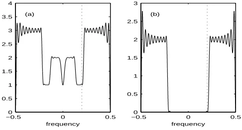
−0.5 0 0.5 0

0.5 1 1.5 2 2.5 3 3.5 4

frequency (a)

−0.5 0 0.5

0 0.5 1 1.5 2 2.5 3

frequency (b)

Fig. 1. (a)SZ(f)and (b)RZ(f).The vertical dotted line marks the frequencyf= 0.2.

VIII. SIMULATIONRESULTS

For p ≥2 we will show that using the scaled F approximation test where we reject H0f in (23) if (46) holds brings about a worthwhile accuracy improvement over Box’s approximation test where we

rejectH0f if

M(f)> K K−pχ

2

2p2(1−α). (47)

To be able to do this we need to simulate from a model such that SU(f) in (7) has RZ(f) =0 for

some frequency range. We can proceed as follows.

We know [30] that any complex second-order stationary scalar process (assumed zero mean here),

whether proper or improper, can be written as the output of a widely linear filter driven by proper white

noise, i.e.,

Zt=

∞

∑

l=−∞

glϵt−l+

∞

∑

l=−∞

hlϵ∗t−l, (48)

where {gl} and {hl} are sequence of complex constants, and {ϵt} is proper white noise for which

cov{ϵt+τ, ϵt} = σϵ2δτ,0 and cov{ϵt+τ, ϵ∗t} = 0, for τ ∈ Z, where δj,k is the Kronecker delta. For simulation purposes it is convenient to set σ2_ϵ = 1.Then [30]

SZ(f) = |G(f)|2+|H(f)|2 (49)

RZ(f) = G(f)H(−f) +G(−f)H(f), (50)

where G(f) is the frequency response function of{gl}given by G(f) =

∑_∞

f

(p, K) 100α% 0.06 0.12 0.18 0.24 0.42

(2,6) 1% 1.5 1.5 1.4 31.1 35.4

1.1 1.1 0.9 25.8 30.0

5% 6.1 6.2 6.3 60.0 63.6

5.0 5.1 5.2 55.3 59.3

(3,8) 1% 2.0 2.1 2.2 55.7 58.9

0.9 1.1 1.1 42.3 45.5

5% 8.2 8.3 8.3 81.0 82.9

4.9 5.1 5.2 72.6 75.2

TABLE II

REJECTION PERCENTAGES OVER10 000REPETITIONS. THE TOP LINE OF EACH ENTRY IS FORBOX’Sχ2APPROXIMATION (38)AND THE LOWER LINE IS FOR THEFAPPROXIMATION OF(46).

For p≥2 we generate processes {Zj,t}, j = 1, . . . , p, such that

Zj,t =

∞

∑

l=−∞

glϵj,t₋l+

∞

∑

l=−∞

hlϵ∗_j,t−l

+

∞

∑

l=−∞

al¯ϵj,t−l+

∞

∑

l=−∞

al¯ϵ∗j,t−l, (51)

where the 2p processes {{ϵj,t},{ϵj,t¯ }, j = 1, . . . , p} are all independent of each other. The filter {gl}

was chosen to be low-pass with a frequency transition zone[0.125,0.15].The filter{hl} was of

‘Hilbert-type’ or all-pass in the frequency zone [0.05,0.45]. Thus G(f) is real and symmetric while H(f) is

imaginary and skew-symmetric. According to (50), if using just these two filters, the resultingRZ(f) is

zero forf ∈[−0.5,0.5].However, the filter{al}was chosen to be high-pass abovef = 0.2and therefore

generates non-zero RZ(f) values at these high frequencies. The resulting SZ(f) andRZ(f) are shown

in Fig. 1.

The matrix SZ(f) is thus of the form SZ(f) = SZ(f)Ip with frequency dependence as shown in Fig. 1(a) while RZ(f) is of the form RZ(f) = RZ(f)Ip with frequency dependence as shown in Fig. 1(b). We can thus simulate from this model to evaluate our hypothesis tests, knowing that for

frequencies whereRZ(f) =0 in factSZ(f)̸=0 and thus (27) is well-defined.

Sample results are shown in Table II for (p, K) = (2,6)and (3,8).So here K= 6 and 8 are indeed

small. HereN = 512 but smaller time series lengths such as 128 produced very similar results. Shown

(H0f in (23) is true) and the latter two are for frequencies where RZ(f) ̸= 0 (H0f is false) — see Fig. 1(b). The top line of each entry is for Box’s χ2 approximation (47) and the lower line is for theF approximation of (46). We see that, proportionately, the latter has a much more accurate rejection rate

than Box’s approximation when H0f is true, but is slightly less accurate when H0f is false. IX. OVERALLTEST

A. Background

Plotting M(f) againstf and identifying frequencies where the critical value is exceeded is potentially

quite informative. Of course, by the definition of propriety, for an overalltest we need to test H0 in (2).

Here the test domain is finite, while for the alternativerZ,τ =0 for allτ ∈Z,the test domain is infinite. However,f ∈[0, f_N]is still a continuum.

The approach taken in [36] is to construct a single test statistic from GLRTs conducted at frequencies

where the spectral estimators are approximately independent, (spaced apart by the frequency bandwidth

of the spectral estimator). However if, say,RZ(f)̸=0for a narrow band of frequencies midway between

two of the testing frequencies, i.e., on the edge of the bandwidths for two of the independent statistics,

the test would be expected to be quite problematic.

Rather than requiring independent statistics we prefer the flexibility of a multiple hypothesis testing

approach. As a proxy for the formal overall test we consider testing the set ofL null hypotheses

Hl:RZ(fl) =0 forf1, . . . , fL, (52)

where {fl} is a set of frequenciesdensely sampling the positive Nyquist range.

B. Controlling the FWER

The familywise error rate (FWER) is defined asPr(V ≥1)whereV is the number of false rejections.

Following [18], let P₍₁₎ <· · ·< P_(L) denote the ordered p-values corresponding to the L tests defined by (52). Let H₍₁₎, . . . , H_(L) be the associated null hypotheses. Let J be the minimal index such that P_(j) > α/[L+ 1−j]. Reject only the null hypotheses H₍₁₎, . . . , H_(J−1). If J = 1 then do not reject any hypotheses; if no such J exists, reject all hypotheses. Then FWER ≤ α. The tests need not be

independent.

C. Controlling the FDR

Controlling the FWER is equivalent to making it unlikely that even one false rejection is made. A

α= 0.05 frequency interval 0.005 0.01 0.02 FWER 4.7 5.0 4.8

FDRi 4.8 5.2 4.9 FDRd 1.0 1.2 1.2

TABLE III

RATES ACHIEVED(PERCENTAGES)OVER10 000REPETITIONS.

proportion of rejections that are incorrect. Then FDRdef=E{FDP}. As before let P₍₁₎ < · · · < P_(L) denote the ordered p-values. Define li = iα/[CLL] and R = max{i : P(i) < li}. Here CL = 1 for independent tests and CL=

∑L

i=11/i, for dependent tests. Let ℓ=P(R),and

reject all null hypothesesHi for whichPi≤ℓ, (53)

then FDR≤α. The independent tests approach is also valid for some forms of positive correlation [3].

The non-unity adjustment CL for dependent tests is general: the level of dependency does not matter;

as a result, this procedure is rather conservative. Nevertheless [3], the dependent tests approach can still

prove much more powerful than the comparable FWER. Note that CL changes as more/less tests are

made (L increases/decreases) or the sampling rate of the frequency range is increased/decreased.

D. Simulation of overall test for true null

Here we will look at an example of when the null hypothesis (2) is true. We use the simulation

set-up of Section VIII for p = 2 but setting the coefficients {al} to zero in (51). Hence RZ(f) = 0

for f ∈ [−0.5,0.5]. With N = 512 and K = 6 the bandwidth of the spectral window (16) is about

0.014. Over the range f ∈[0.02,0.48]we consider three frequency samplings: steps of 0.005, 0.01 and

0.02; the first two are within the spectral window bandwidth and the latter outside, so we would expect

the tests to be dependent for the first two cases, and independent for the third. We carry out 10 000

independent repetitions with α = 0.05 and from these calculate (a) the FWER, and (b) the FDR under

assumptions of (i) independence (FDRi) and (ii) dependence (FDRd). p-values are calculated via the

scaled F approximation. The results are given in Table III. We see thatFWER≤α, as required. (The

test does not require independence.) For FDRi there is variation about 5% in line with the assumed

independence being false for frequency intervals 0.01 and 0.005. FDRd can be seen to be always quite

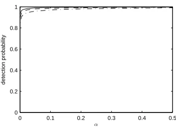
0 0.1 0.2 0.3 0.4 0.5 0

0.2 0.4 0.6 0.8 1

α

detection probability

Fig. 2. The ROC curve for the model of Section IX-E. On the x-axis isα and we are using FDRd. The y-axis gives the probability of detection of impropriety. The curves are forσ2

λ= 0.4(solid), 0.5 (dashed) and 0.6 (dash-dot).

E. Simulation of overall test for false null (ROC curve)

We now consider behaviour when the null hypothesis (2) is false. To illustrate the receiver operating

characteristic (ROC) we use a signal structure used in [27] and [33]. Consider the scalar process Zt=

Xteiλt +ξt where {Xt} is a real-valued stationary zero mean Gaussian process with autocovariance sX,τ = e−τ

2_/5

, λtis a random sequence drawn from a Gaussian distribution with mean zero and variance

σ2

λ,and{ξt} is proper complex-valued Gaussian noise with variance unity. All three random sequences are independent. So the signal-to-noise ratio is unity and the signal is improper [27], [33] while the

noise is proper, as in [36]. A p = 2 vector-valued process was created from two independent copies of

{Zt}. Fig. 2 shows the probability of detection of impropriety (constructed from 10 000repetitions) as a

function of α using FDRd. With N = 1000and K = 12 the bandwidth of the spectral window (16) is

about 0.013, and we sampled the frequencies at an interval of 0.005. The curves are for σ2

λ = 0.4,0.5

and 0.6. Asσ2

λ increases,|RZ(f)|decreases towards zero, and impropriety is increasingly hard to detect.

X. DATAANALYSIS

A. Background

We apply our results to ocean current speed and direction time series recorded at a mooring in the

Labrador Sea [8], [21], [22]. We associate the eastward (zonal) measurement of current speed with{Xt}

and the northward (meridional) measurement with{Yt} and thus obtain the complex-valued series from

(3). We consider series recorded at the three depths 110, 760 and 1260m. The series are labelled 1 to 3

with increasing depth, giving Zt= [Z1,t, Z2,t, Z3,t]T.We used N = 1600observations for the 3 -vector-valued complex time series, with a sampling interval of ∆t= 1hr. In the spectral analysisK = 12 sine

statistical results for a finite-N sample is given by 0.004≤ |f| ≤0.496c/hr. For this data there was no

evidence to reject stationarity [7, p. 49], [8] or Gaussianity [9].

Of great interest to oceanographers are deep ocean motions well away from boundaries, especially in

the internal wave frequency band. We pay special attention to low frequenciesf ∈[0.02,0.14]c/hr within

which interesting rotational effects have been observed in previous studies [8], [38]. The very dominant

semi-diurnal tide at aroundf = 0.08c/hr was estimated and removed to avoid spectral leakage.

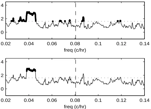
By way of example Fig. 3 shows the scalar quantities SZ(f)andRZ(f) for one of the series. We see

that SZ(f) is asymmetric about f = 0 as expected. For frequencies around f = 0.04c/hr, we see that

|Im{RZ(f)}| is noticeably larger than |Re{RZ(f)}|;these frequencies are of interest later (see Fig. 4).

B. Testing for Propriety

Fig. 4 shows propriety-testing results for our region of interest f ∈ [0.02,0.14]c/hr. The upper plot

shows the test statistic M(f) and the critical value for α = 0.05 for the frequency-specific propriety

test for the vector Zt = [Z1,t, Z2,t, Z3,t]T. On a frequency-by-frequency basis rejection occurs at all frequencies where M(f) exceeds the critical value; these frequencies are shown by heavy dots. The

lower plot shows the results from the overall FDRd approach. Frequencies causing rejection according

to (53) are also marked by heavy dots. As might be expected, the frequencies leading to the overall

rejection of propriety — those around f = 0.04c/hr — are a subset of those causing rejection on a

frequency-by-frequency basis.

We also implemented the testing approach of [36] using — in order to get independent statistics

— multitaper estimates spaced apart by the bandwidth, 0.008c/hr, of the spectral window. Again, with

α = 0.05, overall propriety was rejected, as would be expected given that our test identified the band

of frequencies around 0.04c/hr as responsible for rejection, and this would be easily ‘seen’ with a

frequency spacing of 0.008c/hr. Note, the information conveyed in Fig. 4 is clearly useful in specifying

the frequencies causing rejection, whereas the approach in [36] provides only a decision on propriety. In

situations where isolated narrow bands of frequencies might cause rejection the approach in [36] could

be problematic, as explained in Section IX-A.

XI. SUMMARY ANDCONCLUSION

We have developed a frequency domain approach to test for propriety of complex-valued vector time

series. For the vector case(p≥2)we have justified use of the rule that the frequency-specific hypothesis

H0f in (23) is rejected ifM(f) =−2KlogT(f)> bFν1,ν2(1−α).There is no assumption thatKis large,