Improvement in Large Signal Stability Using PSO Algorithm

(1)

Page 209

Improvement in Large Signal Stability Using PSO Algorithm

M.Divya Sanjana

1

_{, T.R.Jyothsna}

2

PG Student [Power Systems], Dept. of EEE, Andhra University, Visakhapatnam, India

1

Professor, Dept. of EEE, Andhra University, Visakhapatnam,

India

2

---

Abstract

Transient stability of power systems becomes a major factor in planning and day-to-day operations and there is a need for fast on-line solution of transient stability to predict any possible loss of synchronism and to take the necessary measures to restore stability. Recently various controller devices are designed to damp these oscillations and to improve the system stability, which are found in modern power systems, but power system stabilizer (PSS) still remains an attractive solution.

These PSS are local controllers on the generators. Thus local controllers are used to mitigate system oscillation modes. In multi machine system with several poorly damped modes of oscillations, several stabilizers have to be used and the problem of synthesis of PSS parameters becomes relatively complicated. Population based optimization techniques have been applied for PSS design. Studies have revealed that these optimization techniques have improved the system stability.

A population based algorithm called Particle Swarm Optimization (PSO) has been proposed in this thesis for optimal tuning of the power system stabilizer (PSS) for a single machine infinite bus (SMIB) system and 3-machine 10 bus system. Recent studies in artificial intelligence demonstrated that the PSO optimization technique is a powerful intelligent tool for complicated stability problems. This algorithm is based on intelligent behavior of honey bee swarm. The PSS parameters of an SMIB system and 3 machine 10 bus system are tuned to improve large signal stability and eigen values of the system. It is relevant from the results that the proposed PSO algorithm is superior to any conventional technique.

Key Words

:

Particle Swarm Optimization (PSO), Single Machine Infinite Bus (SMIB).

---*---I.INTRODUCTION**

1.1 POWER SYSTEM STABILIZER

Power System stabilizers have been in use for many years as a solution to the problem of oscillatory instability. The PSS, which acts as supplementary modulation controller in the excitation system of generator, produce a component of electrical torque on the rotor Speed. As the objective of PSS is to introduce a damping torque component, the most appropriate signal is the speed deviation. For any input signal, the transfer function of the stabilizer must compensate for the gain and phase characteristics of the excitation, the generator, the power system, which collectively determine the transfer function from stabilizer output to the component of electrical torque which can be modulated via excitation control. This transfer function is strongly influenced by voltage regulator gain, generator power level, and AC system Strength [3].

The control signals for PSS must satisfy the following requirements [4]:

 The signal must be easily synthesized from the locally available measurements.

 To avoid the introduction of filters, the noise content in chosen signal must be minimal.

 The design based on a particular signal must be robust and reject noise.

The basic function of PSS is to add damping to both local and inter – area modes without compromising the stability of other modes.

II. Particle Swarm Optimization

(2)

Page 210

called lbest. when a particle takes all the population as its

topological neighbours, the best value is a global best and is called gbest.The particle swarm optimization concept consists of, at each time step, changing the velocity of (accelerating) each particle toward its pbest and lbest locations (local version of PSO). Acceleration is weighted by a random term, with separate random numbers being generated for acceleration toward best and lbest locations. In past several years, PSO has been successfully applied in many research and application areas. It is demonstrated that PSO gets better results in a faster, cheaper way compared with other methods.

In PSO, each single solution is a particle in the search space. Each individual in PSO flies in the search space with a velocity, which is dynamically adjusted according to the flying experience of its own and its companions. PSO is initialized with a group of random particles. Each particle is treated as a point in a D-dimensional space. The ith particle is represented as xi = (xi1, xi2, . . ., xiD). The best previous position of the ith particle that give the best fitness value is represented as pi = (pi1, pi2, . . ., piD). The best particle among all the particles in the population is represented by pg = (pg1, pg2, . . ., pgD). Velocity, the rate of the position change for particle i is represented as vi = (vi1, vi2, . . . , viD). In every iteration, each particle is updated by following the two best values. After finding the aforementioned two best values, the particle updates its velocity and positions according to the following equations:

viD(new)=viD(old) + c1 r1(piD − xiD) + c2 r2(pgD − xiD) (3.12)

xiD(new)=xiD(old) + viD(new) (3.13)

where c1 and c2 are two positive constants named as learning factors, r1 and r2 are random numbers in the range of (0,1). _ is a restriction factor to determine velocity weight. Eq. (3.12) is used to calculate the particle’s new velocity according to it’s previous velocity and the distances of its current position from its own best position and the group’s best position. Then, the particle flies toward a new position according to Eq. (3.13). Such an adjustment of the particle’s movement through the space causes it to search around the two best positions. If the minimum error criterion is attained or the number of cycles reaches a user-defined limit, the algorithm is terminated.

2.2 Parameter selection

1. Range of the particles

The ranges of the particles depend on the problem to be optimized. One can specify different ranges for different dimension of the particles

2. Maximum velocity vmax

The maximum velocity vmax determines the maximum change one particle can take during one iteration. Usually, the range of the particle is set as vmax. In this work, a

vmax = 4 is chosen for each particle as this gives better optimal results.

3. The inertia parameter

The inertia parameter is introduced by Shi and Eberhart and provides improved performance in a number of applications. It has control over the impact of the previous history of velocities on current velocity and influences the balance between global and local exploration abilities of the particles. A larger inertia weight favors a global optimization and a smaller inertia weight favors a local optimization.

It is suggested to range w in a decreasing way from 1.4 to 0 adaptively. In this work, a constant value of the inertia parameter w = 0.75 is chosen as it facilitates reaching a better optimal value in lesser number of iterations.

4. The parameters c1 and c2

The acceleration constants c1 and c2 indicate the stochastic acceleration terms which pull each particle towards the best position attained by the particle or the best position attained by the swarm. Low values of c1 and c2 allow the particles to wander far away from the optimum regions before being tugged back, while the high values pull the particles toward the optimum or make the particles to pass through the optimum abruptly. If the constants c1 and c2 are chosen equal to 2 corresponding to the optimal value for the problem studied. In the same reference, it is mentioned that the choice of these constants is problem dependent. In this work, c1 = 1 and c2 = 1 are chosen which give better optimal results in lesser iterations.

In a PSO algorithm, multiple candidate solutions called particles coexist and collaborate simultaneously, where each particle denotes a solution X = [x1,x2, . . . ,xN]T. Different from other evolutionary algorithms where the populations are updated by some evolutionary operations, such as cross-over and mutation, each particle in PSO adjusts its position according to its own experience as well as the experience of neighboring particles. Tracking and memorizing the best position encountered build particle’s experience, PSO possesses a memory (every particle remembers the best position it has reached during the past). Especially, PSO combines local search method (through self-experience) with global search methods (through neighboring experience).

III. Implementation of PSO

In this project, PSO with the procedure is summarized as follows:

Step 1: Initialize a population of particles with random positions and velocities, where each particle contains N

(3)

Page 211

Step 2: Evaluate the objective values of all particles, let

pbest of each particle and its objective value equal to its

current position and objective value, and let gbest and its objective value equal to the position and objective

value of the best initial particle.

Step 3: Update the velocity and position of every particle according to Eqs. (3.12) and Eqs (3.13).

Step 4: Evaluate the objective values of all particles. Step 5: For each particle, compare its current objective value with the objective value of its pbest. If current value

is better, then update pbest and its objective value with the current position and objective value.

Step 6: Determine the best particle of current whole population with the best objective value. If the objective value

is better than the objective value of gbest, then update gbest and its objective value with the position and

objective value of the current best particle.

Step 7: If a stopping criterion is met, then output gbest and its objective value; otherwise go back to step (3).

Flow chart

IV. SYSTEM MODEL

In this thesis, the performance of PSS and PSOPSS is compared and analyzed for Single machine infinite bus system (SMIB) and 3-machine system. The gain of the PSS is set by applying particle swarm optimization (PSO) optimization technique. This can enhance the angle stability and provide the voltage regulation at the generator terminals. Transient stability analysis is used to investigate the stability of a power system under sudden and large disturbances with PSS and PSOPSS

3

.1SYSTEM MODEL

3.1.1 Generator Equations

3.1.1.1 Rotor Equations:

The rotor mechanical dynamics for each machine is represented by the swing equations in per unit (p.u) as:

e m 2

2

T

dt

dδ

D

dt

δ

d

M







(3.1)

Where M= 2H/ωB, Tm is the mechanical torque acting on

the rotor, Te is the electrical torque and ωB is the base

synchronous speed. Equation (3.1) can be expressed as two first order equations as:

)

(

m mo

B

S

ω

dt

dδ





(3.2)

H

T

S

D(S

dt

dS

m m mo m e

2 )

)

(









(3.3)

where Sm is generator slip given by

B B m

ω

S





(3.4)

D is p.u damping given by

D



D

'

ωB

. Since the normal operating speed is same as the rated speed, Smo can be

taken as zero.

(4)

Page 212

damper coil on q-axis. Hence, two electrical circuits are

considered on the rotor-a field winding on the d-axis and one damper winding on the q-axis. The resulting equations are:



d fd



' d d ' q ' d0 ' q

E

i

x

E

T

dt

dE

_

_

_

_

_

)

(

1

(3.5)



q



' q q ' d ' q 0 ' d

i

x

E

T

dt

dE

)

(

1 _

_



(3.6) Where q d ' q ' d d ' d q ' q

e

E

i

E

i

x

i

T





(



)

(3.7)

Model (1.0) can be handled by letting q ' q

x



and

0 

' q o

T

. With

E

'_d remaining zero as long as

T

_qo'



0

,

the RHS of equation (3.6) is zero. Hence for model (1.0) equations (3.2), (3.3) and (3.5) apply.

3.1.1.2 Stator equations:

The stator equations in p.u in the d-q reference frame, neglecting the stator transients and variations in the rotor speed, are given by:

d d a q

mo

ψ

R

i

υ

S









(1

)

(3.8)

q q a d

mo

ψ

R

i

υ

S







)

(1

(3.9)

where, Smo is the initial operating slip, q + j d is the

generator terminal voltage and iq + j id is the armature

current, ψqand ψd are the flux linkages in d-q reference

frame. For the 1.1 model of the generator (field circuit with one equivalent damper on the q-axis) the flux linkages are given by:

d ' d ' q d

E

x

i

ψ





(3.10)

' q q ' q q

x

i

E

ψ





(3.11)

Substituting equations (3.10) and (3.11) in (3.8) and (3.9) and letting Smo = 0 we get:

q q a d ' d '

q

x

i

R

i

υ

E







(3.12)

d d a q ' q '

q

x

i

R

i

υ

E





(3.13)

E'd, E'q are equivalent voltage sources for flux linkages

along d i.e. field axis and q axis.

x'd and x'q are transient reactance along d and q axis

respectively.

Equations (3.12) and (3.13) can be combined into a single complex equation as:

d q d q ' a ' d '

q

j

E

R

j

x

i

j

i

v

j

v

E





(



)(



)





(3.14)

3

.2.2

Excitation System

The main objective of the excitation system is to control the field current of synchronous machine. The field current is controlled to regulate the terminal voltage of the machine. As field current time constant is high, field current requires forcing. Thus exciter ceiling voltage should be 5-6 times normal. AVR also results in negative damping thus making the system unstable. The instability is due to exciter mode, is called oscillatory instability. The Automatic Voltage Regulator (AVR) with single time constant is considered. Vg is the terminal voltage, Vs is the

output of the PSS. The state equations for the excitation system is given by



(

)



1

s g ref A fd A fd

V

K

E

T

dt

dE

_

_

_

_

_

fdmax fd

fdmin

E



(3.15)

Where

V

_g



υ

_q2



υ

_d2

3.2 DESIGN OF PSS

3.2.1 PSS Model

Power system stabilizers are supplementary controllers in the excitation system meant to provide damping for generator rotor oscillations. This is necessary as high gain AVRs can contribute to oscillatory instability in the power systems, which are characterized by low frequency oscillations (0.2 to 2.0 Hz). Figure 3.2 shows the block diagram of dynamic compensator of PSS. The washout circuit is provided to eliminate the steady bias in the output of the PSS. The time constants T1 and T2 of the

dynamic compensator; mp denotes the number of stages of

(5)

Page 213

Washout circuit Dynamic compensator smax

V

Smin V w W sT sT  1 p m 1 1 _        2 1 S sT sT K

[image:5.595.35.222.474.579.2]

 ΔVpss

Figure 3.2: Block diagram of PSS

The overall PSS transfer function including the washout circuit is p m 2 1 w w pss

sT

1 sT

K

s

PSS

_





























)

(

(3.19)

The time constant Tw of the washout circuit can be chosen

in the range of 1 to 2 secs,

3.2.2 Objective function

The appropriate value of the PSS gain Ks is obtained by applying nonlinear constrained optimization method. The design of PSS is carried out in two steps. In the first step, independent design of the dynamic

compensators of PSS is accomplished by the method of residues and in the second step, the tuning of the gain of PSS is achieved by the application of nonlinear

constrained optimization algorithm as defined below:

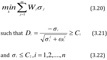
j m

j j

k

W

σ

min



1

(3.20)

such that

C

1

ω

σ

D

2 i 2 i i i









(3.21)

and

σ

i



C

2

,

i



1,2,....

,

n

(3.22)

where m = total number of modes of interest,

n = total no. of eigenvalues,

σi = real part of the ith eigenvalue,

ωi= imaginary part of the ith eigenvalue,

Di = Damping ratio of the ith eigenvalue,

Wj = positive weight associated with the jth swing mode,

k = vector of control parameters, where each of the elements of the vector is greater than zero.

SMIB system data:

Generator data: Base 1000MVA, 400 KV

Bus 1

Ra 0.00327

xd 1.7572

xd’ 0.4245

Tdo’ 6.66

xq 1.5845

xq’ 1.04

Tqo’ 0.44

H 3.542

D 0

Network data:R1 = 0.04296,Xl = 0.40625,Bc = 0.1184,

Xt = Xbr = 0.13636

AVR data:Ka = 200,Ta = 0.05,Efdmax = 6.0,Efdmin = -6.0

Initial operating point:Pg= 0.6,Qg= 0.02224,Vg= 1.05,θ =

21.65o _,E_b_{= 1.0}

3 machine 10 bus systems:

Generator data:

B u s R a x d x d’ T d o’ x q x q’ T q o’

H D K

A

T

A

1 0 0

. 1 4 6 0 0 . 0 6 0 8 8 . 9 6 0 0 0 . 0 9 6 9 0 . 0 9 6 9 0 . 3 1 0 0 2 3 . 6 4 0 0 0 . 0 0 0 0 2 0 0 0 . 0 5 0 0

2 0 0

(6)

Page 214

5 8 9 8 0 0 4 5 6 9 5 0 0 0 0 0 0 0

3 0 1

. 3 1 2 5 0 . 1 8 1 3 5 . 8 9 0 0 1 . 2 5 7 8 0 . 2 5 0 0 0 . 6 0 0 0 3 . 0 1 0 0 0 . 0 0 0 0 2 0 0 0 . 0 5 0 0

Network data

: Data given below is are p.u on a common base of 100MVA

Bus

Nos

Resistance Reactance Shunt

Susceptance

(total)

1 4 0.0000 0.0576 0.0000

4 6 0.0170 0.0920 0.1580

6 9 0.0390 0.1700 0.3580

9 3 0.0000 0.0536 0.0000

9 8 0.0119 0.1008 0.2090

8 7 0.0085 0.0720 0.1490

7 2 0.0000 0.0625 0.0000

10 5 0.0160 0.0805 0.1530

7 10 0.0160 0.0805 0.1530

5 4 0.0100 0.0850 0.1760

Load flow data:

Bu s Volta ge Angle (degre Genera ted Genera ted Load Real Load Reacti

es) Real

Power Reactiv e Power Pow er ve Power

1 1.040

0

0.0000 2.9328 0.9792 0.00

00

0.000

0

2 1.025

3

-1.8240

2.2109 0.5317 0.00

00

0.000

0

3 1.025

3

-8.4708

1.1232 0.3589 0.00

00

0.000

0

4 0.999

0

-9.3571

0.0000 0.0000 0.00

00

0.000

0

5 0.970

2

-16.803

9

0.0000 0.0000 2.25

00

0.750

0

6 0.948

2

-16.916

1

0.0000 0.0000 1.90

00

0.600

0

7 1.002

0

-9.5538

0.0000 0.0000 0.00

00

0.000

0

8 0.969

1

-15.441

1

0.0000 0.0000 2.00

00

0.650

0

9 1.006

8

-12.126

4

0.0000 0.0000 0.00

00

0.000

0

V. RESULT AND DISCUSSION

(7)

Page 215

critically dependent upon the magnitude, nature and the

location of fault and to a certain extent on the system operating conditions. The stability analysis of the system under such conditions, normally termed as ‘transient-stability’ analysis is generally attempted using mathematical models involving a set of non-linear differential equations.

4.3 Transient Stability

analysis

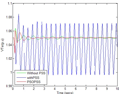
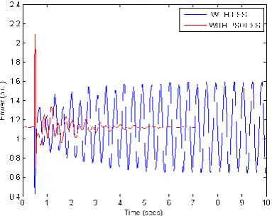
The system behavior is analyzed for three phase fault. The three phase fault is created on the critical bus 7 with a line outage. The fault is initiated at 0 sec and is cleared within 2.5 sec. The output of PSS can regulate the exciter voltage as a result of which the real power output of the machines and also the bus voltage variation at the critical buses have also reduced as shown in Figures. From the results it is clear that oscillations are damped and the system is stabilized at a faster rate compared to the conventional PSS. Here, PSS is placed at third generator.

4.3.1 Results for transient stability:

Fig 4.1: Variation rotor angle without PSS, with PSS and

with PSOPSS for SMIB

Fig 4.1: Variation rotor angle without PSS, with PSS and

with PSOPSS for 3machine systems

Fig 4.2: Variation in terminal voltage without PSS, with

[image:7.595.323.552.110.295.2] [image:7.595.313.557.361.554.2] [image:7.595.47.269.443.619.2]

(8)

[image:8.595.50.283.111.290.2]

Page 216

Fig 4.2: Variation in terminal voltage without PSS, with

PSS and with PSOPSS for 3machine systems

Fig 4.3: Variation in torque for SMIB system without PSS,

with PSS and with PSOPSS

Fig 4.4: Variation in power for 3machine system without

PSS, with PSS and with PSOPSS

VI.CONCLUSION

This chapter has presented the Particle Swarm Optimization Algorithm for the design of power system stabilizers. The performance evaluation of the proposed stabilizer on a single machine system shows that increased robustness could be achieved by application of PSO to stabilizer design. The design procedure using PSO is also simple and can be used for particle implementation. The performance of the PSOPSS is compared with CPSS. PSOPSS gives better performance compared to CPSS.

R

EFERENCES

[1] P.Kundur, Power System Stability and Control,

McGraw-Hill Press 1994.

[2] P.M.Anderson and A.A.Fouad Power System Control

and Stability, Iowa State University Press, Ames, Iowa,

1977.

[3] E.V Larsen and D.A. Swann, “Applying power system

stabilizers: Parts I, II, III, “IEEE Transactions on power

apparatus and systems, vol. PAS-100, PP.

3017-3046’1981.

[4] K.R. Padiyar, Power System Dynamic-Stability and

Control, BS Publications, Hyderabad, India, 2006.

[5] K. R. Chowdhury, M. Di Felice, “Search: a routing

protocol for mobile cognitive radio ad hoc networks,”

Computer Communication Journal, vol. 32, no. 18, pp.

1983-1997, Dec.20

[6] K. M. Passino, “Biomimicry of bacterial foraging for

distributed optimization,” IEEE Control Systems

Magazine, vol. 22, no. 3, pp. 52-67, 2002.

[7] Q. Wang, H. Zheng, “Route and spectrum selection in

dynamic spectrum networks,” in Proc. IEEE CCNC

2006, pp. 625-629, Feb. 2006.

[8] R. Chen et al., “Toward Secure Distributed Spectrum

Sensing in Cognitive Radio Networks,” IEEE Commun.

Mag., vol. 46, pp. 50–55, Apr. 2008.

[9] H. Khalife, N. Malouch, S. Fdida, “Multihop cognitive radio networks: to route or not to route,” IEEE Network, vol. 23, no. 4, pp. 20-25, 2009.

[image:8.595.45.292.351.466.2] [image:8.595.49.241.529.681.2]

Improvement in Large Signal Stability Using PSO Algorithm

Page 209