Analysis of Rainfall Intensity Duration Frequency Relationship for Rwanda

http://dx.doi.org/10.4236/jwarp.2016.87058

How to cite this paper: Wagesho, N. and Claire, M. (2016) Analysis of Rainfall Intensity-Duration-Frequency Relationship for Rwanda. Journal of Water Resource and Protection, 8, 706-723. http://dx.doi.org/10.4236/jwarp.2016.87058

Analysis of Rainfall

Intensity-Duration-Frequency Relationship

for Rwanda

Negash Wagesho

, Marie Claire

1_{Department of Water Resources & Irrigation Engineering, Arba Minch University, Arba Minch, Ethiopia} 2_{Ministry of Defense, Kigali, Rwanda}

Received 23 March 2016; accepted 13 June 2016; published 16 June 2016

Copyright © 2016 by authors and Scientific Research Publishing Inc.

This work is licensed under the Creative Commons Attribution International License (CC BY).

http://creativecommons.org/licenses/by/4.0/

Abstract

Global atmospheric and oceanic perturbations and local weather variability induced factors highly alter the rainfall pattern of a region. Such factors result in extreme events of devastating nature to mankind. Rainfall Intensity Duration Frequency (IDF) is one of the most commonly used tools in water resources engineering particularly to identify design storm event of various magnitude, duration and return period simultaneously. In light of this, the present study is aimed at develo- ping rainfall IDF relationship for entire Rwanda based on selected twenty six (26) rainfall gauging stations. The gauging stations have been selected based on reliable rainfall records representing the different geographical locations varying from 14 to 83 years of record length. Daily annual maximum rainfall data has been disaggregated into sub-daily values such as 0.5 hr, 1 hr, 3 hr, 6 hr and 12 hr and fitted to the probability distributions. Quantile estimation has been made for dif- ferent return periods and best fit distribution is identified based on least square standard error of estimate. At-site and regional IDF parameters were computed and subsequent curves were estab-lished for different return period. The moment ratio diagram (MRD) and L-moment ratio diagram (LMRD) methods have been used to fit frequency distributions and identify homogeneous regions for observed 24-hr maximum annual rainfall. The rainfall stations have been divided into five homogeneous rainfall regions for all 26 stations. The results of present analysis can be used as useful information for future water resources development planning purposes.

Keywords

Intensity, Duration, Frequency, Maximum Rainfall, Regionalization, Rwanda

1. Introduction

Highly induced atmospheric water vapour content as result of raising global temperature resulted in increased maximum precipitation. The increasing precipitation intensity and magnitude is recognized to have a significant impact on disaster management efforts and pose challenging threat towards the efforts to meet the growing needs of the most vulnerable population in sub-Saharan parts of Africa.

Rainfall Intensity-Duration-Frequency (IDF) relationship is one among the plethora of tools used for planning, designing and operating water resource development infrastructures [1][2]. It gives an idea on return period of rainfall intensity which can be expected within a defined period [3]-[7]. It also provides a concise information between the maximum intensity of rain that falls within a given period of time [8]-[10]. Annual maxima and magnitudes above certain threshold or partial duration series of rainfall data are commonly applied as input for IDF analysis [11]. Bougadis and Adamowski [12] used scale invariance concept of rainfall events to disaggre-gate rainfall data from low resolution to high resolution for use in intensity-duration-frequency analysis. Cheng & Agha Kouchak [13] argues that stationary time series assumption may reduce the extreme precipitation mag-nitude and ultimately increases the flood risk.

Hydrological information like IDF relationship being the principal input of design of sewer systems and other hydraulic structures is not yet readily available in systematically organized relationships to the end users in Rwanda. The lack of systematic relationships between events leads the design of many water resources infra-structures to be based on inadequate and unreliable data and information. Therefore, drainage system and high-ways fail to accommodate the unprecedented flood magnitude and easily get ruined.

Rwanda known for land of thousand hills whereby non-uniform topographical formation coupled with man- induced activities favored the local fluctuations in rainfall pattern across the country. This in turn resulted in de-vastating flood destruction over the past couples of years. The country suffered serious floods, landslides and drought events linked to ENSO (El Niño Southern Oscillation) episodes. The 1997/1998 high rainfall devoured planation and resulted in other associated environmental damages. Similarly the 1999/2000 drought episode sig-nificantly affected the Bugesera, Umutara and Mayaga regions [14]. Heavy rainfall, in combination with natural factors like steep topography, resulted in significant socio-economic impacts in the country [15].

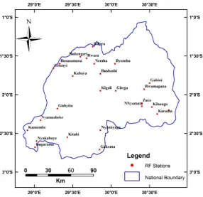
The present study is aimed at developing comprehensive IDF relationship for twenty six (26) selected meteo-rological stations in Rwanda (Figure 1) and clustering rainfall stations into homogeneous regions based on

24-hrs annual maximum rainfall depth.

2. The Study Area

Rwanda is a small landlocked country in East African Great Lakes region. It lies within latitudes 1˚S - 3˚S and longitudes 28˚E - 31˚E having surface area of 26,338 km2. It is bordered with Uganda in the north and Tanzania in the east while in the south and west are Burundi and the Democratic Republic of Congo, respectively. The recent Population of Rwanda is growing fast and counts around 12 million according to the National Institute of Statistics of Rwanda. The divide between two of Africa’s great watersheds, the Congo and Nile basins, extends from north to south through western Rwanda at an average elevation of 2743 meters [15]. Agriculture being the mainstay of the majority of the rural population, erratic equatorial rainfall pattern endangered the agricultural production. Even though Rwanda is situated in the equatorial rain-forest belt, it perceives a modified humid cli-mate characterized by both equatorial rainforest and savannah type. The rainfall pattern is dominated by the subtropical anticyclone as a consequence of the Inter Tropical Convergence Zone positions permitting bimodal rainfall pattern to the region. Majority of the eastern belts of the country receive low seasonal rainfall and are characterized as drought prone areas.

3. Materials and Methods

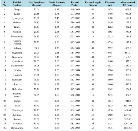
Short to long period (14 - 83 years) daily observed rainfall records have been collected from Rwanda Meteoro-logical Agency under Ministry of Natural Resources. The concise information of rainfall stations considered for present analysis are presented in Table 1. The rainfall data at each stations has undergone through preliminary data scrutiny for consistency. Using stations spatial proximity principle missing daily rainfall records are ac-counted. Maximum daily rainfall magnitudes are disaggregated into sub-daily values of 0.5 hr, 1 hr, 3 hr, 6 hr and 12 hr. Multiples of probability distributions are used to fit the sample data for selected rainfall durations so as to reinforce the statistical argument. In this case, Normal distribution, Extreme Value-I distribution, two pa-rameter Gamma distribution, Log Pearson Type III distribution and two papa-rameter Log-normal distribution are used. Moment ratio diagram (MRD) and L-moment ratio diagram (LMRD) techniques are used to estimate pa-rameters of the distribution and test the goodness of fit of probability distributions. The best fitted probability distribution is utilized to estimate the quantile estimates for different return period. Based on regional homo-geneity analysis, stations having similar rainfall pattern are identified and the entire country is divided into five homogenous daily maximum rainfall zones.

3.1. IDF Curve Parameter Estimation

The intensity-duration-frequency relationship is established for each station and parameters of IDF curves are identified using the following relationship.

The typical generalized IDF parameters can be estimated using the following relationship [16].

(

)

a I

t γ

=

+ (1)

where I = maximum intensity (mm/hr); t = rainfall duration (min.); α = regression coefficient (mm/hr); γ = time constant (min) and c = exponent with values less than unity. In Equation (1) the constants γ and c do not depend on return period, however, the constants vary significantly with location and estimated for specific region. Con-verting Equation (1) into logarithmic form and reducing the sum of the squared deviation to minimum, we have,

(

)

ln I= lnα− ∗C ln t+γ (2)

(

)

{

}

(

)

1

ln ln ln

n

i

S I a C t γ

=

 

=

∑

Equation (2) and (3) are utilized to compute the required intensities for respective stations and durations.

3.2. Quantile Estimation

Table 1. Typical characteristics of rainfall stations under consideration. S. No. Rainfall Stations East Longitude (Degree) South Latitude (Degree) Record Period Record Length (Years) Elevation (m) Mean Annual RF (mm)

1 Gitega 30.06 1.95 1969-2014 46 1474 1069.7

2 Kigali 29.86 1.95 1971-2014 43 1490 1069.5

3 Nyamiyaga 29.86 2.46 1957-2013 57 1800 1198.1

4 Gakoma 29.85 2.71 1986-2013 28 1450 1159.2

5 Kitabi 29.43 2.55 1984-2014 31 2262 1832.2

6 Gishyita 29.30 2.18 1981-2014 32 1665 1539.5

7 Busasamana 29.33 1.60 2001-2014 14 2055 1114.3

8 Gisenyi

Airport 29.25 1.66 1982-2014 33 1554 1112.1

9 Kabaya 29.5 1.76 1974-2014 41 2292 1000.8

10 Bugarama 29.01 2.68 1981-2014 34 900 897.3

11 Kamembe 28.91 2.46 1971-2014 44 1591 1500.3

12 Nyakabuye 29.03 2.60 1997-2014 18 1400 1527.0

13 Nyamasheke 29.08 2.33 1977-2014 38 1527 1317.6

14 Nemba 29.78 1.60 1987-2014 28 1686 1535.7

15 Rushashi 29.86 1.73 1979-2012 32 1650 1259.5

16 Ruhengeri 29.60 1.51 1952-2014 63 1860 1399.6

17 Rwaza 29.68 1.53 1932-2014 83 1800 1332.2

18 Bulera lac 29.76 1.38 1947-2014 68 1862 1134.7

19 Byumba

meteo 30.05 1.60 1996-2014 19 2235 1332.5

20 Gahini 30.5 1.85 1974-2014 41 1534 1016.5

21 Zaza 30.41 2.11 1945-2014 70 1515 1138.60

22 Nyarubuye 30.75 2.20 1958-2013 56 1750 924.08

23 Kibungo 30.53 2.16 1957-2012 56 1680 1097.15

24 Karama 30.60 2.25 1965-2014 50 1347 915.66

25 Nyamata 30.45 2.15 1982-2014 33 1428 1084.79

26 Rwamagana 30.43 1.93 1950-2014 63 1535 1115.83

1 1

F T

= − (4)

where F is the probability of an event having a magnitude of XT or less and the T-years magnitude is given by:

1 2

T T

X =µ +K ∗µ (5)

where KT is the frequency factor which is a function of return period and the parameter of the distribution and μ1 and μ2 are the moments of the distribution. The point estimate of certain quantile corresponding to a return pe-riod may be insignificant unless there is a proof of estimate of accuracy. The validity of estimated quantile checked by the standard error of estimate, ST.

( )

T T T

S = _X −E X _ (6)

3.3. Regionalization Rainfall Frequency Analysis

The observed at-site hydrologic time series data are very short in length and hence substituting space for time is deployed to obtain representative average information about the region. The regional frequency analysis based on index flood method [17][18], L-moments [19]-[22], region of influence [23], canonical correlation analysis [24] and others have been in use in literature. In the present study, the method suggested by Hosking and Wallis [25] is applied to identify candidate homogenous regions for maximum daily rainfall magnitudes. Invariant sta-tions are identified by discordance measure. The MRD and LMRDs are estimated for all station based on the 24-hr maximum rainfall magnitude. Regionalization was made on statistical values (Cs, Ck, LCs, LCk) of maximum rainfall of the selected duration for each station based on the concept that stations in the same region are assumed to be drawn from similar parent distribution. Thus, similarity of the stations (Cs, Ck) and (LCs, LCk) plots to the theoretical probability distributions is accounted to classify the stations and determine the best fitting probability distribution helpful for subsequent quantile estimation.

4. Results and Discussion

4.1. Estimation of IDF Parameters

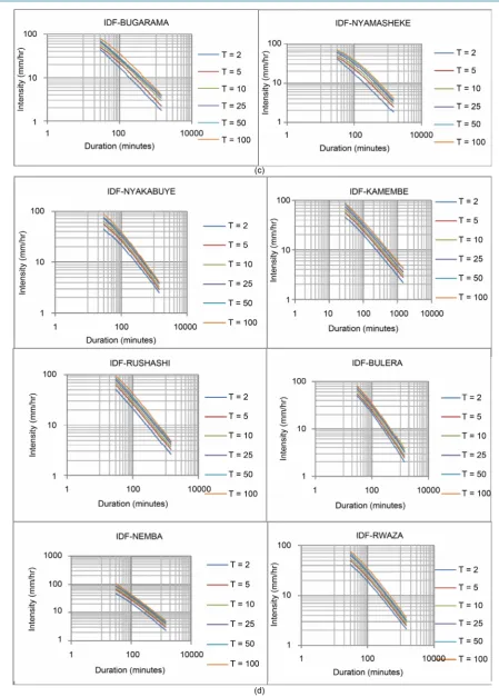
As available data in majority of the rainfall stations is daily record, reducing the available data in manageable sub-daily scale has been carried out using the uniform random disaggregation model. The disaggregated sub- daily data is further statistically checked against the historical records for corresponding duration. It has been found that there is no statistically significant variability between the desegregated and historical observations for selected stations. The IDF parameters are computed for all 26 stations for return period of 2, 5, 10, 25, 50 and 100 years. The computed IDF parameters are presented in Table 2. The parameters exhibit similarity over return period, however, there is no well-defined relationship with respect to station location. The IDF curves have been developed for all station for different return period (Figure 2). To aid water resources planners and decision

Table 2. Computed IDF parameters for selected (15) stations.

S.N Stations Coefficiens T = 2 yrs T = 5 yrs T = 10 yrs T = 25 yrs T = 50 yrs T = 100 yrs

1 Bugarama

α 1048.23 1650.65 1289.53 1109.04 1057.19 2169.15

γ 6.38 17.33 11.71 4.85 2.19 15.94

C 0.88 0.91 0.83 0.79 0.77 0.86

SEE 1.82 0.56 2.53 2.32 2.00 1.55

2 Bulera

α 2250.96 2142.42 2480.84 2268.19 2846.76 2017.67

γ 20.56 19.80 19.57 17.33 18.55 11.71

C 0.97 0.93 0.94 0.90 0.93 0.86

SEE 1.84 1.84 1.81 2.11 1.84 2.49

3 Busasamana

α 1123.60 1373.92 1544.18 1831.31 2214.25 2532.86

γ 0.62 2.44 3.15 3.94 6.43 8.62

C 0.80 0.80 0.80 0.82 0.84 0.84

SEE 0.77 0.83 0.79 0.95 0.78 1.28

4 Byumba

α 2155.87 1222.45 1078.97 1018.31 1068.94 1187.06

γ 28.94 11.58 4.85 0.05 0.02 0.02

C 0.95 0.85 0.82 0.80 0.79 0.80

SEE 1.84 1.77 2.13 3.18 3.15 2.62

5 Gahini

α 366.08 2122.56 2206.10 2259.42 2460.77 2435.12

γ 0.00 22.42 20.56 18.55 16.85 13.71

C 0.68 0.91 0.92 0.91 0.92 0.91

Continued

6 Gakoma

α 653.46 745.76 814.81 980.55 1037.34 1232.85

γ 0.02 0.05 0.05 0.05 0.05 0.62

C 0.78 0.76 0.76 0.77 0.76 0.77

SEE 4.44 4.02 4.31 4.41 4.49 3.90

7 Gisenyi

α 713.11 780.93 898.91 1231.39 1322.68 2015.57

γ 0.62 0.62 0.62 2.19 0.62 6.38

C 0.80 0.76 0.76 0.79 0.78 0.83

SEE 4.52 3.28 3.70 1.74 2.67 2.36

8 Gishyita

α 743.60 1045.55 841.99 923.06 958.47 1029.51

γ 4.25 7.38 2.03 2.00 0.62 0.62

C 0.80 0.83 0.78 0.78 0.77 0.77

SEE 2.87 3.04 2.79 3.20 2.99 3.00

9 Gitega

α 1351.90 1200.76 2087.7 2301.76 2533.42 2153.77

γ 13.94 7.63 13.14 10.25 9.23 4.22

C 0.90 0.86 0.93 0.93 0.93

SEE 1.17 1.29 1.21 1.04 0.93

10 Kabaya

α 2312.29 1427.51 1482.56 1571.987 2369.535 2520.63

γ 26.03 11.85 8.32 3.94 11.86 8.61

C 0.97 0.87 0.86 0.85 0.88 0.88

SEE 2.48 1.74 1.28 1.94 0.91 1.18

11 Kamembe

α 1222.07 1241.79 1181.43 1387.63 1199.10 1888.25

γ 13.94 8.61 4.61 4.85 0.62 8.22

C 0.86 0.84 0.81 0.81 0.77 0.83

SEE 1.5228 2.4225 2.8966 3.3448 4.1961 2.9383

12 Karama

α 3525.93 3669.83 3419.79 3510.284 3648.82 3728.63

γ 47.83 45.31 35.89 29.36 27.42 23.03

C 0.98 0.98 0.97 0.97 0.97 0.96

SEE 1.69 1.63 1.39 0.95 0.81 0.68

13 Kibungo

α 3600.71 3617.14 3219.35 3564.30 3723.39 3729.97

γ 46.59 43.12 32.25 27.41 24.18 20.54

C 0.97 0.97 0.95 0.95 0.95 0.95

SEE 2.67 2.48 1.97 1.73 1.55 1.39

14 Kigali

α 1040.31 1592.58 2130.82 3047.59 4010.53 5792.70

γ 7.79 10.70 14.94 21.54 27.79 37.88

C 0.86 0.91 0.930 0.95 0.96 0.99

SEE 1.34 2.02 1.17 0.35 0.67 1.35

15 Kitabi

α 1526.31 2708.73 3153.95 3665.86 4547.55 4377.41

γ 13.94 28.94 29.49 29.02 32.27 29.37

C 0.89 0.93 0.94 0.94 0.96 0.94

Figure 2. MRD and LMRD for 24 hrs maximum annual rainfall data.

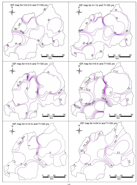
makers, the interpolated IDF map is prepared for entire Rwanda based on 24-hrs annual maximum rainfall dis-tribution for selected return period (Figure 3). These maps will assign particular rainfall intensity magnitude to particular points over the study area through spatial interpolation.

4.2. Fitting Probability Distribution

The 24-hrs annual maximum rainfall magnitude is subjected to MRD (Ck versus Cs) and LMRD (LCk versus LCs) plot whereby station information close enough to the theoretical distribution is assumed to fit the data well. Based on LMRD analysis, the General Logistic and General Extreme value distributions fits well for about 80% of the stations. However, Pearson type-III, General logistic and Gamma distribution put in the front list for MRD case for majority of the stations (Figure 4). A diagram based on Cs & Ck and LCs & LCk are used to identify the appropriate distribution that fits therainfall data. But L-moment ratios plot well separated and al-lows identifying of distribution.

4.3. Regional Rainfall Frequency Analysis

The conventional MRD and LMRD are primarily used to identify homogeneous regions for 24-hr annual maxi-mum rainfall distribution. The L moment ratios (LCs and LCk) for each station based on specific duration rain-fall is plotted against its regional averages on L-moment ratio diagrams. It is assumed that LCs, LCk values of one station varies linearly with LCs, LCk values of the neighboring station. A suitable parent distribution is that which averages the scattered data and around which the data spread consistently. The delineation result indi-cated that five (5) homogeneous regions were established. The transect starts with region-1 in the North-west part of the country and extends progressively to region-5 in the South-east parts in the transverse direction. Re-gion 1 includes the Bulera, Byumba, Nemba, Ruhengeri, Rushashi and Rwaza stations whereby the Generalized Logistic distribution fits well. This region covers a very limited North-west part of the country. Region-2 covers the Busasamana, Gisenyi, gishyita and Kabaya stations residing to the south of region-1.The Bugarama, Ca-membert, Kiitabi, Nyamasheke and Nyakabuye stations are categorized under region-3. Region-4 accounts for Gakoma, Gitega, Kigali and Nyamiyaga stations. All other stations are grouped into region 5, the south western region (Figure 5). The regression coefficient, α decreases as one moves from region-1 to region-5. The rainfall stations grouped into particular regions and corresponding best fitting distributions are listed in Table 3.

(d)

Figure 5. Homogeneous regions identified based on rainfall frequency analysis.

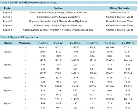
Table 3. LMRD and MRD based station clustering.

Region Stations Fitting Distribution

Region-1 Bulera, Byumba, Nemba, Ruhengeri, Rushashi and Rwaza Generalized logistic

Region-2 Busasamana, Gisenyi, Gishyita and Kabaya Gamma & Pearson Type-II

Region-3 Bugarama, Kamembe, Kitabi, Nyamasheke and Nyakabuye Generalized extreme Value

Region-4 Gakoma, Gitega, Kabaya, Kigali and Nyamiyaga Generalized extreme Value

Region-5 Gahini, Karama, Kibungo, Nyarubuye, Nyamata, Rwamagana and Zaza Gamma & Pearson Type-II

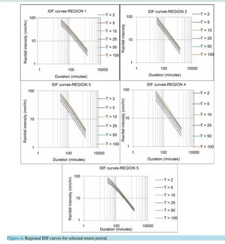
Table 4. Regional IDF parameters.

Region Parameters T = 2 yrs T = 5 yrs T = 10 yrs T = 25 yrs T = 50 yrs T = 100 yrs

Region 1

α 1649.52 1737.75 1847.72 1894.85 1895.00 2278.12

γ 20.56 17.33 15.92 13.14 10.09 13.67

C 0.91 0.89 0.88 0.86 0.85 0.86

Region 2

α 983.74 1112.82 1095.21 1375.48 1566.78 1861.69

γ 4.85 4.85 2.20 3.15 3.15 4.85

C 0.83 0.81 0.79 0.81 0.82 0.83

Region 3

α 976.75 1390.01 1401.19 1590.16 1784.72 2237.48

γ 10.62 15.94 13.85 13.70 14.96 17.33

C 0.84 0.86 0.84 0.84 0.84 0.86

Region 4

α 724.64 847.46 994.08 1076.6 1133.46 1983.76

γ 3.15 2.36 3.15 2.19 0.62 9.23

C 0.79 0.78 0.78 0.77 0.76 0.83

Region 5

α 729.58 976.10 1145.79 1389.89 1690.38 1661.38

γ 3.09 4.85 4.85 5.62 7.29 4.84

Figure 6. Regional IDF curves for selected return period.

Table 5. Regional quantile (mean of stations) for the selected duration.

Return Period 0.5 hr 1 hr 3 hr 6 hr 12 hr 24 hr

2 yr 23.1 31.8 38.9 45.7 50.5 52.5

5 yrs 27.9 38.2 46.1 54.7 60.0 65.0

10 yrs 31.5 42.9 51.4 60.8 68.7 73.1

25 yrs 36.1 48.4 57.6 68.7 77.7 83.7

50 yrs 40.2 52.8 62.7 74.0 84.9 91.4

5. Conclusions

Theoretical probability distribution for the 24-hr annual maximum rainfall depths for different durations has been selected using moment ratio and L-moment ratio diagrams methods. Based on the least standard error of estimate, best fitted probability distributions are identified and subsequent quantiles have been computed for different return period. Rainfall IDF parameters for selected duration and recurrence interval are computed for all stations under consideration. The adequacy of computed rainfall intensities are evaluated through statistical analysis against the observed values. The results of these tests indicated that the estimated IDF parameters ade-quately represented the rainfall intensities for most of the stations.

Rainfall station clustering has been made taking into account the annual maximum rainfall depth of 24-hr du-ration. The best fitted distribution for each homogeneous regions were identified based on statistical values of LCs and LCk of annual maximum rainfall depth for all implied stations. Based on MRD and LMRD analysis, the rainfall stations are categorized into five homogeneous regions. The rainfall stations clustered within a re-gion sufficiently satisfied the homogeneity test. Identified rere-gional parameters are representative of the at-site information for longer rainfall durations, however, deviation from the regional parameters is observed for short-er rainfall duration in some regions.

Available automatic rainfall stations are very limited in number and most of the regions have got a short rain-fall record (less than five years). Therefore, developing IDF map from existing information through statistical analysis may be subjected to imprecision and prone to certain errors. Future water resources planning and design studies should rely on reliable observed rainfall data from automated stations to develop IDF maps.

References

[1] Mohymont, B.G. (2004) Establishment of IDF-Curves for Precipitation in the Tropical Area of Central Africa. Natural

Hazards and Earth System Sciences, 4, 375-387. http://dx.doi.org/10.5194/nhess-4-375-2004

[2] Lam, K. (2004) Update of the Short Duration Rainfall IDF Curves for Recent Climate in Quebec. Canadian water Res.

Assoc. Ann. cong.

[3] Koutsoyiannis, D.K. (1998) A Mathematical Framework for Studying Rainfall Intensity-Duration-Frequency Rela-tionships. Journal of Hydrology, 206, 118-135. http://dx.doi.org/10.1016/S0022-1694(98)00097-3

[4] Koutsoyiannis, D. (2003) On the Appropriateness of the Gumbel Distribution for Modelling Extreme Rainfall. Pro-ceedings of the ESF LESC Exploratory Workshop, Hydrological Risk: Recent Advances in Peak River Flow Model-ling, Prediction and Real-Time Forecasting, Assessment of the Impacts of Land-Use and Climate Changes, European Science Foundation, National Research Council of Italy, University of Bologna, Bologna.

[5] Nhat, L., Tachikawa, Y. and Takara, K. (2006) Derivation of Rainfall Duration Frequency Relationship for Short Du-ration Rainfall from Daily Rainfall. Proc. of Int.l Symp. on Managing Water Supplyfor Growing Demand, Technical

Document in Hydrology, 6, 89-96.

[6] Prodanovic, P. and Simonovic, S.P. (2007) Development of Rainfall Intensity Duration Frequency Curves for the City of London Under the Changing Climate. Water Resources Research Report No. 058, Facility for Intelligent Decision Support, Department of Civil and Environmental Engineering, London, Ontario, Canada, 51 p.

[7] Khalid, K. and Elsebaie, I. (2013) Development of Intensity Duration Frequency Relationship for Abha City in Saudi Arabia. International Journal of Computer Engineering Research, 3, 58-65.

[8] Bernard, M. (1932) Formulas for Rainfall Intensities of Long Duration. Trans.ASCE, 96, 592-624.

[9] Chow, V., Maidment, D. and Mays, L. (1988) Applied Hydrology. McGraw-Hill Book Company, New York.

[10] De Paola, F., Giugni, M., Topa, M.E. and Bucchignani, E. (2014) Intensity Duration Frequency (IDF) Rainfall Curves, for Data Series and Climate Projection in Africa Cities. Springer Plus, 3, 133.

http://dx.doi.org/10.1186/2193-1801-3-133

[11] Ben-Zvi, A. (2009) Rainfall Intensity-Duration-Frequency Relationships Derived from Large Partial Duration Series.

Journal of Hydrology, 367, 104-114. http://dx.doi.org/10.1016/j.jhydrol.2009.01.007

[12] Bougadis, J. and Adamowski, K. (2006) Scaling Model of Rainfall Intensity-Duration-Frequency Relationship.

Hy-drological Processes, 20, 3747-3757. http://dx.doi.org/10.1002/hyp.6386

[13] Cheng, L. and Agha Kouchak, A. (2014) Nonstationary Precipitation Intensity-Duration-Frequency Curves for Infra-structure Design in a Changing Climate. Scientific Reports, 4, 7093, 1-6.

[15] REMA, Ruwanda Environmental Managemnent Authority (2006) Rwanda State of Environment and Outlook. Kigali.

[16] Wenzel Jr., H.G. (1982)Rainfall for Urban Stormwater Design,Urban Stormwater Hydrology, Water Resour. Monogr., 7D. F. Kibler, AGU, Washington DC.

[17] Dalrymple, T. (1960) Flood Frequency Analysis. US Geological Survey. Water Supply Paper, 1543 A.

[18] Grover, P.L., Burn, D.H. and Cunderlik, J.M.A. (2002) Comparison of Index Flood Estimation Procedures for Un-gauged Catchments. Canadian Journal of Civil Engineering, 29, 734-741. http://dx.doi.org/10.1139/l02-065

[19] Hosking, J.R.M. (1990) L-Moments: Analysis and Estimation of Distributions Using Linear Combinations of Order Statistics. Journal of the Royal Statistical Society, Series B, 52, 105-124.

[20] Atiem, A. and Harmancioglu, N.B. (2006) Assessment of Regional Floods Using L-Moments Approach: The Case of the River Nile. Water Resources Management, 20, 723-747. http://dx.doi.org/10.1007/s11269-005-9004-0

[21] Gonzalez, J. and Valids, J.B. (2008) A Regional Monthly Precipitation Simulation Model Based on an L-Moment Smoothed Statistical Regionalization Approach. Journal of Hydrology, 348, 27-39.

http://dx.doi.org/10.1016/j.jhydrol.2007.09.059

[22] Saif, B. (2009) Regional Flood Frequency Analysis Using L-Moments for the West Mediterranean Region of Turkey.

Water Resources Management, 23, 531-551. http://dx.doi.org/10.1007/s11269-008-9287-z

[23] Burn, D.H. (1988) Delineation of Groups for Regional Flood Frequency Analysis. Journal of Hydrology, 104, 345-361.

http://dx.doi.org/10.1016/0022-1694(88)90174-6

[24] Cavadias, G.S. (1989) Regional flood Estimation by Canonical Correlation. Paper Presented to the 1989 Annual Con-ference of the Canadian Society for Civil Engineering, St-John’s, Newfoundland.