ISSN: 1992-8645 www.jatit.org E-ISSN: 1817-3195
5070
IMAGE SEGMENTATION BASED ON LOCAL SIMILARITY
FACTOR FOR UNEVEN ILLUMINATED IMAGES
R.PRADEEP KUMAR REDDY1,DR. C. NAGARAJU2
1Assistant Professor, Department of CSE, Y.S.R.Engineering College of YVU, India
2Associate Professor, Department CSE, Y.S.R.Engineering College of YVU, India
E-mail: 1[email protected], 2[email protected]
ABSTRACT
In many of the applications the content of an uneven illuminated images needs to be improved or recognized. For the degraded source images the global thresholding algorithm fails to produce adequate results. Due to this reason many applications used local thresholding techniques to binarize each pixel based on gray scale information of its neighborhood pixels. This paper discusses about the design and development of local thresholding techniques using specific fuzzy inclusion and entropy measures with fixed ‘r’ and variable ‘r’. The noise influence on thresholding also tested using different noises like salt & pepper, Gaussian and speckle noises at different proportions. Different statistical parameters are evaluated to test the performance of the local thresholding algorithm with fixed ‘r’ and variable ‘r’. It is evidenced from the results that the local thresholding method with variable ‘r’ produced better results than compared to other methods.
Keywords: Non-uniform Illumination, Global Thresholding, Local Thresholding, Fuzzy Inclusion, Entropy Measures.
1. INTRODUCTION
The research into the image binarization can be traced back to the pioneering work on global threshold based methods, such as the famous Otsu’s method. But this assumption is hardly satisfied in most real applications, especially to camera-captured document images. To overcome the disadvantage of single global threshold binarization method researchers often use the adaptive threshold or local threshold which computes the threshold of each pixel according to the properties of its own or its neighbor pixels.
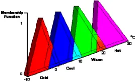
[image:1.612.353.491.413.496.2]Fuzzy is built based on set of rules supplied by user further these rules are converted into mathematical equations. This simplifies role of designer and results are in form of more accurate representation. Fuzzy set theory is invented by Lofti Zadeh [1] from California University in 1965. He proposed a paradigm consisting set of rules and regulations are used to define boundaries. These boundaries represent successful solution for a given problem. The natural phenomena of fuzzy logic is defined in the following figure.
Figure 1: Fuzzy sets to characterize the temperature of the room.
The process of encoding the image data in fuzzy theory called as Fuzzification. The reverse process of encoding often referred as defuzzification between these two an intermediate stage is represented in fuzzy image processing referred as modification of membership value.
Figure 2: Fuzzy histogram hyperbolization image enhancements.
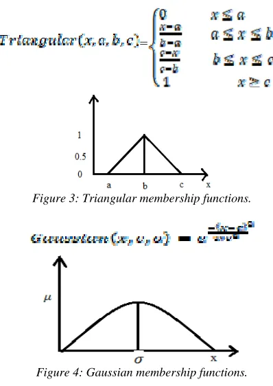
[image:1.612.319.515.600.646.2]5071 triangular and Gaussian membership functions. The basic definitions of these functions defined as
=
[image:2.612.91.290.124.405.2]Figure 3: Triangular membership functions.
Figure 4: Gaussian membership functions.
Depending on the membership function and its shape fuzzifier change the values this process is done by hedge operator. In order to implement a fuzzy set with set of pairs the membership value is defined or modified using hedge operator. Sample version of fuzzy-set defined as
=
Hedge operator operates on membership function which may result reducing or increasing the contrast of image depending on the value contained at that position. The hedge operator also may also used to change the quality of the image.
The new grey level values are generated for given image by the image defuzzification using modified values of membership function. This process also uses fuzzy histogram hyperbolization. This process modifies membership values of grey level pixels by using a logarithmic equation is.
Where, μmn ( ) is the grey level in the fuzzy membership values,
β is hedge operator, and is the new grey level value
Due to uneven or bad illumination, the intensity of background is not consistent within the camera-captured document image which causes the single threshold based method impractical. In the implementation of fuzzy logic various thresholds are considered but existing methodology used global thresholding for reasons global thresholding has failed in image segmentation. The failures of global thresholding defined as [3]:
1. Global thresholding fails when there is a low contrast foreground and background. 2. It fails when image is consisting noise 3. It fails when intensity of background
changes across the image.
To overcome above failures a new methodology is proposed using fuzzy sets by considering fixed and variant membership values.
2. LITERATURE REVIEW
Image
segmentation
is an essential stage of image processing which divides the input image into connected regions, homogeneous and non-overlapping [4]. This indicates that any two spatially separated neighborhood regions are inhomogeneous. [5]. Many techniques have been proposed by the researchers; however, no technique is suggestible to use for all images which gives satisfactory results [6].Generally, image pixels are the property of a particular region and each region of the pixels in the image should be homogeneous with reference to selected characteristics such as intensity or texture. Every region should have the property of non-overlapping or connectivity. Non-non-overlapping region is the essential property where the any two pixels corresponding to that region should be connected in line and further it should not leave the region. Merging of neighborhood regions may not create a single homogeneous region. Thresholding is a process of converting the images from grayscale to binary which creates foreground and background objects from the original and complementary states respectively. Some of the applications use gray level-0 (black) for foreground objects and highest luminance (white) for document paper (i.e 255 in 8-bit images) or vice versa [7].
mean-ISSN: 1992-8645 www.jatit.org E-ISSN: 1817-3195
5072 deviation. From the results they observed that the determination of mean is independent of window size. They also reported that as compared to other local thresholding methods the proposed method speeds up the process.
Bogiatzis et al [9] discussed a method used to binarize the unevenly illuminated texts using specific fuzzy inclusion and entropy measure techniques. They discussed that the whole process is automated and is an open procedure which with further research can be generalized in order to be effective on “difficult” images of different domains and of various characteristics.
3. IMPACT NOISE IN IMAGE
Different types of noises are introduced in the digital images at different stages of the pre-processing which degrades the images. Such degradation influences negatively the performance of many image processing methods. Hence in many of techniques it is prerequisite to include a filter module before processing the digital image which is contaminated with the noise [10, 11]. The challenge of many image processing technologies is to suppress the noise as well to preserve the true edges and detailed information of the image.
3.1. Impulse Noise
Due to non-uniformness in the image noise corrupts the original pixels. This noise is caused due to sensors, hardware and transmission of data in noise channels. It is classified into two types like fixed impulse and random impulse. The fixed impulse is popularly known as salt and pepper noise. This noise appears like as black and white speckles in image. This noise is corrupts higher extreme or lower extreme intensity values. Therefore, degradation is automatically applied to image causes for non-identity of objects in the image.
The noise image model for impulse noise as follows.
Where f(x, y) is the original image pixel, η(x, y) is the noise term and g(x, y) is the resulting noisy pixel.
3.2. Gaussian Noise
Generally, images are corrupted with different types of noises. Among them one of the noise is Gaussian noise which is an additive noise to an image. But due to power in the bandwidth
Gaussian is added naturally such noise is called as additive white Gaussian noise. This noise is independent to intensity of gray level value at each point. The main sources of occurring the Gaussian noise is data acquisition, high temperature and transmission. The mathematical model of additive white Gaussian noise as follows.
Where g = gray value, s = standard deviation and μ = mean.
3.3. Speckle Noise
This noise is modelled with value of random multiplications with respect to pixel in the image which can be expressed in term of
P = I + n * I
Where P indicates the distribution of noise in the image, I is input image and n is uniform noise in the image with respect to mean and variance. Generally, this noise is observed in remote sensing system due to the radiation in sensing the image using laser light and interaction of target area.
4. PROPOSED METHOD
The transition of proposed method is generation of local threshold instead of using the global threshold for image segmentation. Bogiatzis and Papadopoulos [12, 13] is used a set of measure of fuzzy set defined as S1 but in the proposed process a fuzzy set S2 is measured completely equivalent to S1. Let us consider a pixel P with m×n neighbourhood n is a fuzzy set using S1, S2 is measured with a proper subsets defined between set n and set x as
= (X, A), = (A,∅), = (P, A ), = (A, P)
Entropy is measured for n using E1, let us consider that e = E1(N). The entropy is calculated as similar process of second implementation using fuzzy sets according to the values of s1 and s2. With the above referred algorithm following groups are formed.
5073 -Group 6 N with > and 0.5 < | − | ≤ 0.75 -Group 7 N with > and 0.25 < | − | ≤ 0.5 -Group 8 N with > and | − | ≤ 0.25
Steps involved in multi scale edge detection using random fuzzy sets
1. Let us consider an image with m×n each pixel intensity of image is divided into 255, which generates a fuzzy sets N.
2. Consider X as universal set with same size of input image consisting white image.
3. Construct Ø as a Dark image which is a complement of X, which is defined ØϵXc.
4. Construct P as a Gray image with respect to x. 5. X is a finite set and A, B are two sets which are
defined with membership functions mA(x) and mB(x).
6. Construct random sets S1, S2, S3 and S4 with the help of fuzzy inclusion between set A and sets X,
∅
and P.7. Here S1 indicates brightness of the image S2 indicates darkness, S3 and S4 measured as greyness of image.
8. Further calculate entropy with respect to membership function A. where e = E1(A). 9. Compute r as a fuzzy set, which can be
estimated in two methods
a) First implementation of algorithm with respect to fixed values.
b) A second implementation of our algorithm where the values of r is a random values, but they are computed depending on the values of s1 and s2. 10. Estimate fuzzy symmetric triangular number as
t = (r-c, r, r+c) Where C = |s3-s4|
11. Consider entropy e as a truth value and compute t1 and t2 as follows
t1=c * (e-1) + r and t2 =c * (1-e) + r
12. Based on the equality criteria i.e either t = t1 or t = t2.
13. Final threshold has been considered to binarize the image
All these functionalities are defined from Young’s axiom theorem.
Fixed ‘r’ implementation for each class
Local thresholding to too complex when compared with global threshold this says that it is essential to cover various and different domains of image to evaluate local threshold. In this first implementation degraded images are considered where illumination is non-uniformly spread over the image. Due to the limitation of global threshold
which is not able to cover overall areas of image local thresholding is evaluated with the help of first and simplest fixed r implementation. In this procedure r is a standardized by defining 8 classes more specifically the 8 classes are defined with lower and higher boundaries using fuzzy sets as follows:
If N belongs to class 1 set r = 0.49 (0.49 − 0.495) If N belongs to class 2 set r = 0.48 (0.48 − 0.49) If N belongs to class 3 set r = 0.47 (0.47 − 0.48) If N belongs to class 4 set r = 0.46 (0.46 − 0.47) If N belongs to class 5 set r = 0.43 (0.43 − 0.44) If N belongs to class 6 set r = 0.44 (0.44 − 0.45) If N belongs to class 7 set r = 0.45 (0.45 − 0.46) If N belongs to class 8 set r = 0.46 (0.46 − 0.47)
If ≤ then t = t1 else t = t2 If t ≤ 0 then t = 0.01 If t ≥ 1 then t = 0.99
Second implementation: varying r for each class Adding sensitivity in automatic fashion is not a easy task which requires a lot of research. In fact, sensitivity parameter needs to improve the binarization factor to achieve flexible segmentation. The set of group of values for second implementation is not fixed they are computed depending on s1 and s2. Specifically, the varying r classes defined as:
If N belongs to class 1 set r = 0.41+ 0.08 s2 If N belongs to class 2 set r = 0.39 + 0.112 s2 If N belongs to class 3 set r = 0.37 + 0.153 s2 If N belongs to class 4 set r = 0.35 + 0.206 s2 If N belongs to class 5 set r = 0.41 + 0.036 s1 If N belongs to class 6 set r = 0.39 + 0.098 s1 If N belongs to class 7 set r = 0.37 + 0.115 s1 If N belongs to class 8 set r = 0.35 + 0.206 s1
5. RESULTS AND DISCUSSIONS
The experimental result is analyzed to assess the efficiency of proposed and existing methods. Efficiency of proposed method is studied by introducing various kinds of noises to the input image. The methods which are proposed provides better results when compared with existing being Gaussian, salt and papper and speckal noise is applied up to some level. The matching parameters
JACCARD, BRUAN, KULCZYNSKI1,
ISSN: 1992-8645 www.jatit.org E-ISSN: 1817-3195
5074 figure 5, 6 and 7. Most of the times the proposed two methods are showing better results when compared with existing method for various matching parameters mentioned above.
Noise Percent
age
Original
Image Method Global Fixed ‘r’ Method Variable
‘r’ Method
0
5
10
15
20
[image:5.612.316.516.80.394.2]25
Figure 5: Input and output images for Salt and Pepper noise.
Noise Percenta
ge
Original
Image Method Global Fixed ‘r’ Method Variable
‘r’ Method
0
5
10
15
20
25
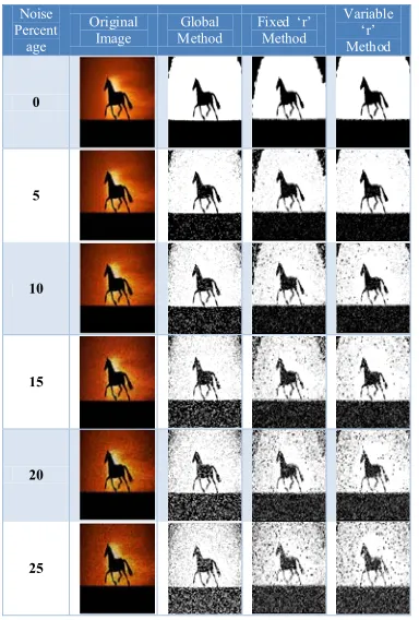
Figure 6: Input and output images for Gaussian Noise.
Noise Percent age
Original
Image Method Global Fixed ‘r’ Method Variable ‘r’ method
0
5
10
15
20
[image:5.612.93.285.149.433.2]25
Figure 7: Input and output images for Speckle Noise
Table 1: Values of JACCARD for Salt and Pepper noise Noise
Percentage Method Global ‘r’ Method Variable Fixed ‘r’ Method
0 0.9320 0.9420 0.9468
5 0.8759 0.8885 0.9000
10 0.8258 0.8385 0.850
15 0.7866 0.7900 0.820
20 0.7500 0.7510 0.757
25 0.7200 0.7280 0.7350
0 0.5 1
0 5 10 15 20 25
JACCARD for Salt & Pepper Noise
Global Method Fixed 'r' Method Variable 'r' Method
[image:5.612.320.513.432.681.2] [image:5.612.93.273.471.710.2]5075 Table 2: Values of JACCARD for Gaussian noise
Noise Percentage
Global Method
Variable ’r’ Method
Fixed ‘r’ Method
0 0.8846 0.9054 0.9273 5 0.7398 0.7758 0.7944 10 0.6390 0.6764 0.6851 15 0.6065 0.6262 0.6362 20 0.5825 0.6074 0.6290 25 0.5162 0.5855 0.6000
0 0.2 0.4 0.6 0.8 1
0 5 10 15 20 25
out
p
ut
v
al
ue
s
Noise Percentage
Jaccard for Gaussian Noise
Global Method Fixed 'r' Method
Variable 'r' Method
[image:6.612.107.281.112.381.2]Figure 9: Graphical Representation of JACCARD for Gaussian Noise
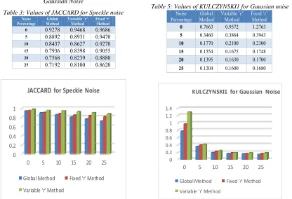
Table 3: Values of JACCARD for Speckle noise Noise
Percentage Global Method
Variable ’r’ Method
Fixed ‘r’ Method 0 0.9278 0.9468 0.9686
5 0.8892 0.8931 0.9470
10 0.8437 0.8627 0.9270
15 0.7936 0.8398 0.9055
20 0.7568 0.8239 0.8880
25 0.7192 0.8100 0.8620
0 0.2 0.4 0.6 0.8 1
0 5 10 15 20 25
JACCARD for Speckle Noise
Global Method Fixed 'r' Method
Variable 'r' Method
Figure 10: Graphical Representation of JACCARD for Speckle Noise
Table 4: Values of KULCZYNSKI1 for Salt & Pepper noise
Noise
Percentage Method Global Variable ’r’ Method Fixed ‘r’ Method
0 1.3716 1.6239 1.7782
5 0.7059 0.7965 0.7965
10 0.4742 0.5193 0.5397
15 0.3686 0.3774 0.3844
20 0.3000 0.3100 0.3500
25 0.2500 0.2600 0.2800
0 0.5 1 1.5 2
0 5 10 15 20 25
KULCZYNSKI1 for Salt & Pepper Noise
Global Method Fixed 'r' method
[image:6.612.328.509.118.375.2]Variable 'r' Method
[image:6.612.104.520.402.686.2]Figure 11: Graphical Representation of KULCZYNSKI1 for Salt &Pepper Noise
Table 5: Values of KULCZYNSKI1 for Gaussian noise
Noise
Percentage Method Global Variable ’r’ Method Fixed ‘r’ Method
0 0.7663 0.9572 1.2763
5 0.3460 0.3864 0.3943
10 0.1770 0.2100 0.2300
15 0.1554 0.1675 0.1748
20 0.1395 0.1630 0.1700
25 0.1204 0.1600 0.1680
0 0.2 0.4 0.6 0.8 1 1.2 1.4
0 5 10 15 20 25
KULCZYNSKI1 for Gaussian Noise
Global Method Fixed 'r' Method
Variable 'r' Method
[image:6.612.315.511.415.689.2]ISSN: 1992-8645 www.jatit.org E-ISSN: 1817-3195
5076 Table 6: Values of KULCZYNSKI1 for Speckle noise
Noise
Percentage Method Global Variable ’r’ Method Fixed ‘r’ Method
0 1.2851 3.0798 3.394
5 0.8028 1.7853 1.9806
10 0.6283 1.2697 1.3101
15 0.5242 0.9577 1.0638
20 0.4677 0.7927 1.0638
25 0.3242 0.6541 0.9890
0 0.5 1 1.5 2 2.5 3 3.5
0 5 10 15 20 25
KULCZYNSKI1 for Speckle Noise
[image:7.612.107.280.124.383.2]Global Method Fixed 'r' Method Variable 'r' Method
[image:7.612.322.513.133.398.2]Figure 13: Graphical Representation of KULCZYNSKI1 for Speckle Noise
Table 7: Values of KULCZYNSKI2 for Salt & Pepper noise
Noise
Percentage Method Global Variable ’r’ Method Fixed ‘r’ Method
0 0.1930 0.1940 0.1990
5 0.1860 0.1870 0.1880
10 0.1800 0.1820 0.1831
15 0.1760 0.1770 0.1780
20 0.1710 0.1720 0.1734
25 0.1642 0.1674 0.1700
0 0.05 0.1 0.15 0.2
0 5 10 15 20 25
KULCZYNSKY2 for Salt & Pepper Noise
lobal Method Fixed 'r ' Method
Variable 'r' Method
Figure 14: Graphical Representation of KULCZYNSKI2 for Salt &Pepper Noise
Table 8: Values of KULCZYNSKI2 for Gaussian noise Noise
Percentage Method Global Variable ’r’ Method Fixed ‘r’ Method
0 0.1881 0.1904 0.1926
5 0.1722 0.1732 0.1794
10 0.1635 0.1650 0.1690
15 0.1607 0.1620 0.1640
20 0.1582 0.1600 0.1630
25 0.1500 0.1550 0.1600
0 0.05 0.1 0.15 0.2
0 5 10 15 20 25
KULCZYNSKY2 for Gaussian Noise
Global Method Fixed 'r' Method
Variable 'r' Method
[image:7.612.102.289.431.704.2]Figure 15: Graphical Representation of KULCZYNSKI2 for Gaussian Noise
Table 9: Values of KULCZYNSKI2 for Speckle noise Noise
Percentage Global Method
Variable ’r’ Method
Fixed ‘r’ Method
0 0.1930 0.1960 0.1971
5 0.1882 0.1900 0.1950
10 0.1824 0.1910 0.1970
15 0.1760 0.1900 0.1930
20 0.1710 0.1850 0.1900
25 0.1600 0.1800 0.1887
0 0.05 0.1 0.15 0.2
0 5 10 15 20 25
KULCZYNSKI2 for Speckle Noise
Global Method Fixed 'r' Method
[image:7.612.120.505.434.699.2]ariable 'r' Method
[image:7.612.327.511.443.692.2]5077 Table 10: Values of BRAUN for Salt & pepper noise
Noise Percentage
Global Method
Variable ’r’ Method
Fixed ‘r’ Method
0 0.9590 0.9655 0.9704
5 0.9211 0.9319 0.9373
10 0.8849 0.8941 0.9040
15 0.8464 0.8577 0.8704
20 0.8000 0.8100 0.8221
[image:8.612.102.289.111.363.2]25 0.7794 0.7900 0.7997
[image:8.612.331.504.112.367.2]Figure 17: Graphical Representation of BRAUN for Salt &Pepper Noise
Table 11: Values of BRAUN for Gaussian noise
Noise Percentage
Global Method
Variable ’r’ Method
Fixed ‘r’ Method
0 0.8982 0.915 0.9388
5 0.7434 0.7816 0.7955
10 0.6416 0.6772 0.6852
15 0.6091 0.6262 0.6363
20 0.5826 0.6200 0.6300
25 0.5500 0.6000 0.6200
0 0.2 0.4 0.6 0.8 1
0 5 10 15 20 25
BRAUN for Gaussian Noise
Global Method Fixed 'r' Method
[image:8.612.106.285.402.675.2]Variable 'r' Method
Figure 18: Graphical Representation of BRUAN for Gaussian Noise
Table 12: Values of BRAUN for Speckle noise
Noise Percentage
Global Method
Variable ’r’ Method
Fixed ‘r’ Method
0 0.9594 0.9765 0.9811
5 0.9365 0.9565 0.9655
10 0.9143 0.9375 0.9436
15 0.8942 0.9166 0.9292
20 0.8795 0.8991 0.9069
25 0.8512 0.8732 0.8923
0.75 0.8 0.85 0.9 0.95 1
0 5 10 15 20 25
BRAUN for Speckle Noise
Global Method Fixed 'r' Method
Variable 'r' Method
Figure 19: Graphical Representation of BRAUN for Speckle Noise
Table 13: Values of DICE for Salt & Pepper noise Noise
Percentage Method Global Variable ’r’ Method Fixed ‘r’ Method
0 0.4000 0.5000 0.7218
5 0.4360 0.4408 0.6869
10 0.4150 0.4200 0.6558
15 0.3720 0.3920 0.6270
20 0.3280 0.3561 0.6067
25 0.3070 0.3323 0.5859
0 0.2 0.4 0.6 0.8
0 5 10 15 20 25
DICE for Salt & Pepper Noise
Global Method Fixed 'r' Method
Variable 'r' method
[image:8.612.331.508.411.677.2]ISSN: 1992-8645 www.jatit.org E-ISSN: 1817-3195
[image:9.612.107.284.98.381.2]5078 Table 14: Values of DICE for Gaussian noise
Noise
Percentage Method Global Variable ’r’ Method Fixed ‘r’ Method
0 0.3959 0.4711 0.7485
5 0.4019 0.4772 0.7630
10 0.4044 0.4820 0.7659
15 0.4083 0.4832 0.7663
20 0.4094 0.4835 0.7680
25 0.4100 0.4900 0.7800
0 0.5 1
0 5 10 15 20 25
Dice for Guassian Noise
Global Method Fixed 'r' Method Variable 'r' Method
Figure 21: Graphical Representation of DICE for Gaussian Noise
Table 15: Values of DICE for Speckle noise
Noise
Percentage Method Global Variable ’r’ Method Fixed ‘r’ Method
0 0.3820 0.4655 0.7304
5 0.3593 0.4508 0.7008
10 0.3424 0.4306 0.6732
15 0.3276 0.4174 0.6435
20 0.3168 0.3977 0.6192
25 0.3012 0.3870 0.6008
0 0.5 1
0 5 10 15 20 25
DICE for Speckle Noise
[image:9.612.324.509.99.371.2]Global Method Fixed 'r' Method Variable 'r' Method
Figure 22: Graphical Representation of DICE for Speckle Noise
Table 16: Values of SIMPSON for Salt & Pepper noise Noise
Percentage
Global Method
Variable ’r’ Method
Fixed ‘r’ Method
0 0.9707 0.9730 0.9750
5 0.9470 0.9486 0.9501
10 0.9253 0.9259 0.9370
15 0.8960 0.8985 0.9047
20 0.8500 0.8590 0.8900
25 0.8200 0.8300 0.8746
0.7 0.75 0.8 0.85 0.9 0.95 1
0 5 10 15 20 25
SIMPSON for Salt & Pepper Noise
Global Method Fixed 'r ' Method
Variable 'r' Method
[image:9.612.323.512.410.678.2]Figure 23: Graphical Representation of SIMPSON for Salt &Pepper Noise
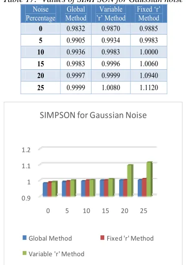
Table 17: Values of SIMPSON for Gaussian noise
Noise Percentage
Global Method
Variable ’r’ Method
Fixed ‘r’ Method
0 0.9832 0.9870 0.9885
5 0.9905 0.9934 0.9983
10 0.9936 0.9983 1.0000
15 0.9983 0.9996 1.0060
20 0.9997 0.9999 1.0940
25 0.9999 1.0080 1.1120
0.9 1 1.1 1.2
0 5 10 15 20 25
SIMPSON for Gaussian Noise
Global Method Fixed 'r' Method
Variable 'r' Method
[image:9.612.107.282.415.695.2]5079 Table 18: Values of SIMPSON for Speckle noise
Noise
Percentage Method Global ’r’ Method Variable Fixed ‘r’ Method
0 0.9658 0.9900 0.9987
5 0.9463 0.9896 0.9934
10 0.9386 0.9881 0.9983
15 0.9324 0.9867 0.9996
20 0.9287 0.9863 0.9999
25 0.9158 0.9857 1.0010
0.86 0.88 0.9 0.92 0.94 0.96 0.98 1 1.02
0 5 10 15 20 25
SIMPSON for Speckle Noise
Global Method Fixed 'r' Value
Variable 'r' Method
[image:10.612.321.510.93.369.2]Figure 25: Graphical Representation of SIMPSON for Speckle Noise
Table 19: Values of ROGERS for Salt & Pepper noise
Noise Percentage
Global Method
Variable ’r’ Method
Fixed ‘r’ Method
0 0.9151 0.9282 0.9346 5 0.8450 0.8623 0.8689 10 0.7822 0.8010 0.8084 15 0.7336 0.7434 0.7479 20 0.6875 0.6957 0.7038 25 0.6503 0.6596 0.6585
0 0.5 1
0 5 10 15 20 25
ROGERS for Salt & Pepper Noise
[image:10.612.109.282.96.371.2]Global Method Fixed 'r' Method Variable 'r' Method
Figure 26: Graphical Representation of ROGERS for Salt &Pepper Noise
Table 20: Values of ROGERS for Gaussian noise Noise
Percentage MethodGlobal Variable ’r’ Method Fixed ‘r’ Method
0 0.8642 0.8785 0.9089
5 0.6453 0.7203 0.7215
10 0.5165 0.5448 0.5531
15 0.4558 0.4655 0.4785
20 0.3859 0.4216 0.4664
25 0.3112 0.3987 0.4587
0 0.2 0.4 0.6 0.8 1
0 5 10 15 20 25
Rogers for Gaussian Noise
Global Method Fixed 'r' Method
Variable 'r' Method
[image:10.612.101.502.409.698.2]Figure 27: Graphical Representation of ROGERS for Gaussian Noise
Table 21: Values of ROGERS for Speckle noise
Noise Percentage
Global Method
Variable ’r’ Method
Fixed ‘r’ Method
0 0.9181 0.9611 0.9650
5 0.8757 0.9351 0.9416
10 0.8473 0.9116 0.9149
15 0.8234 0.8869 0.8977
20 0.8070 0.8674 0.8714
25 0.8000 0.8400 0.8650
0 0.2 0.4 0.6 0.8 1
0 5 10 15 20 25
Rogers for Speckle Noise
Global Method Fixed 'r' Method
Variable 'r' Method
[image:10.612.331.504.409.676.2] [image:10.612.106.285.423.673.2]ISSN: 1992-8645 www.jatit.org E-ISSN: 1817-3195
5080
6. CONCLUSION
Optimal local thresholding technique based on random fuzzy sets and entropy measures is presented for segmenting multiresolution and unevenly illuminated images. The performance of the proposed technique was also studied under the influence of noise on the images. Three different noises were added at different proportions to the original image and vast number of statistical measures were evaluated to understand the performance of the proposed algorithm with fixed and variable ‘r’ value and also compared with existing global method. The methods which are proposed provides better results when compared with existing being Gaussian, salt and pepper and speckle noise is applied up to some level. It efficiently segments the multiresolution image and works well for low contrast and overlapping images.
REFRENCES:
[1] L. A. Zadeh, “Fuzzy sets”, Information and control 8, 338--353 (1965).
[2] Jin Zhao, B.K. Bose, “Evaluation of membership functions for fuzzy logic-controlled induction motor drive”, IEEE 2002 28th Annual Conference of the Industrial Electronics Society. IECON 02.
[3] Ashutosh Kumar Chaubey, “Comparison of The Local and Global Thresholding Methods in Image Segmentation”, World Journal of Research and Review (WJRR), 2(1), 2016 01-04.
[4] A. Usinskas and R. Kirvaitis, “Automatic analysis of hu-man head ischemic stroke: review of methods”, Electronics and Electrical Engineering, Kaunas: Technologija, 7(49), 52 – 59, 2003.
[5] S.M. Bhandarkar and H. Zhang, “Image
Segmentation using Evolutionary
Computation”, IEEE transactions on
Evolutionary Computation, 3(1), 1 – 21, 1999. [6] Bounsaythip, C. and Alander J.T., “Genetic Algorithms in Image Processing - A Review”,
Proc. Of the 3rd Nordic Workshop on Genetic Algorithms and their Applications, Metsatalo, Univ. of Helsinki, Helsinki, Finland, pp. 173-192, 1997.
[7] Mehmet Sezgin and Bu¨ lent Sankur, “Survey over image thresholding techniques and quantitative performance evaluation”, Journal of Electronic Imaging 13(1), (January 2004), pp 146–165.
[8] T.Romen Singh, Sudipta Roy, O.Imocha Singh, TejmaniSinam, Kh.Manglem Singh, “A New Local Adaptive Thresholding Technique in Binarization”, International Journal of Computer Science Issues, 8(6), 271-277, 2011.
[9] Athanasios C. Bogiatzis, and Basil K. Papadopoulos, “Binarization of texts with varying lighting conditions using fuzzy inclusion and entropy measures”, AIP Conference Proceedings 1978, 290006, 2018. [10]M. Tulin Yıldırım, Alper Bas¸ turk and M.
Emin Yuksel, Impulse Noise Removal From Digital Images by a Detail-Preserving Filter Based on Type-2 Fuzzy Logic, IEEE transactions on fuzzy systems, pp-920-928, 2008.
[11]Tom Mélange, Mike Nachtegael, and Etienne E. Kerre, Fuzzy Random Impulse Noise Removal from Color Image Sequences, IEEE transactions on image processing, pp-959-970, 2011.
[12]Bogiatzis A, Papadopoulos B, “Binarization of texts with varying lighting conditions using fuzzy inclusion and entropy measures”, Int Conf Num Anal Appl Math 1978(1), 290006, 2018.