A novel codon based de Bruijn graph algorithm for gene construction from unassembled transcriptomes

M E T H O D

Open Access

A novel codon-based de Bruijn graph

algorithm for gene construction from

unassembled transcriptomes

Gongxin Peng

, Peifeng Ji

and Fangqing Zhao

Abstract

Most gene prediction methods detect coding sequences from transcriptome assemblies in the absence of closely related reference genomes. Such methods are of limited application due to high transcript fragmentation and extensive assembly errors, which may lead to redundant or false coding sequence predictions. We present inGAP-CDG, which can construct full-length and non-redundant coding sequences from unassembled transcriptomes by using a codon-based de Bruijn graph to simplify the assembly process and a machine learning-based approach to filter false positives. Compared with other methods, inGAP-CDG exhibits a significant increase in predicted coding sequence length and robustness to sequencing errors and varied read length.

Keywords:de Bruijngraph, Gene prediction, Phylogenomics, Transcriptome

Background

Gene prediction provides basic functional information for understanding the genome sequence of a species and has become a crucial component of many frameworks used in genomic studies. With the rapid development of sequencing technology, transcriptome sequencing has become an efficient and cost-effective method for gener-ating vast sequencing data for the prediction of genes for phylogenomic studies. Phylogenetically, orthologous genes are defined as genes descended from the sequence of a common ancestor through speciation [1]. The reliable identification of orthologous genes derived from high-quality coding sequences (CDSs) is critical for phylogen-etic tree construction, an important component of many phylogenomic and functional studies. However, orthology inference is especially challenging for datasets reliant on transcriptomes containing misassemblies and partial or missing genes [2]. In particular, in eukaryotic transcrip-tomes, many genes have multiple isoforms, which may result in monophyletic or paraphyletic tips on the phylo-genetic tree. For example, a widely used transcriptome

assembler, Trinity [3], usually assembles many isoform groups (a subcomponent) for a given gene locus.

For species with reference genomes, functional genes are usually predicted using homology-based methods, which can identify genes by aligning target sequences to the original genes of closely related species. However, the reference database only represents a small fraction of existing species, limiting such methods to the se-quences collected. Thus, gene prediction methods rely-ing on known reference genomes limit our functional understanding of novel species. When related reference genomes are lacking, ab initio prediction methods utiliz-ing assembled genomic sequences are inherently difficult due to the quality of training datasets [4–8]. Korf et al. found that in the absence of sufficient training data, GenScan [9] exhibited poor performance, with a sensi-tivity of 22.1% and a specificity of 20.0% for gene prediction in Drosophila melanogaster[7]. Alternatively, gene prediction can be performed based on de novo transcriptome assembly, which can considerably reduce the size of the dataset and increase the functional infor-mation obtained compared with genome sequencing. However, these methods are significantly limited by the quality of de novo transcriptome assembly, which is sensitive to sequencing errors, repetitive sequences in different genes, and the overlap of transcripts encoded * Correspondence:[email protected]

†_{Equal contributors}

1_{Computational Genomics Lab, Beijing Institutes of Life Science, Chinese}

Academy of Sciences, Beijing, China

2

University of Chinese Academy of Sciences, Beijing, China

by adjacent loci [3]. Hence, a typical transcriptome assembly may result in a large set of fragmented, redun-dant, and error-containing transcripts. For instance, an RNA-sequencing (RNA-seq) Genome Annotation Assess-ment Project (RGASP) competition study revealed that the highest accuracy of transcript assembly was only 48% for the RNA-seq reads of three transcriptome datasets [10]. Therefore, orthologous gene datasets derived from assem-bled transcripts are usually incomplete, fragmented, and redundant and often contain errors and isoforms that fun-damentally skew the underlying assumptions of orthology inference in phylogenomic analyses.

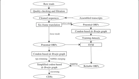
To overcome this difficulty and to increase the utility of transcriptome datasets, we developed inGAP-CDG, an algorithm that can perform gene construction from unassembled transcriptomes. Compared with previous approaches, inGAP-CDG predicts open reading frames (ORFs) directly from unassembled reads, exploits a supervised support vector machine (SVM) to filter false-positive ORFs, and employs a novel codon-based de Bruijn graph to assemble cleaned ORFs into full-length CDSs (Fig. 1). Using both simulated and real datasets, we demonstrated that inGAP-CDG can significantly im-prove the length and precision of gene recognition. inGAP-CDG is implemented in C++ and the source

code is freely available together with full documentation at https://sourceforge.net/projects/ingap-cdg.

Results

Codon-based de Bruijn graph versus traditional de Bruijn graph

As shown in Additional file 1: Supplementary Methods, we have offered mathematical proof demonstrating that the codon-based de Bruijn graph exhibits a substantial advantage over the traditional de Bruijn graph due to a decrease in graph nodes and edges. To further demon-strate this reduction and to quantify the difference between codon-based and traditional graphs, we used both simulated and real datasets to compare their prop-erties. We generated three chr3 Consensus Coding Se-quences (CCDSs) annotated datasets for human, mouse, and fruit fly, respectively. For each dataset, both a traditional graph and a codon-based de Bruijn graph were constructed. The number of nodes and edges in each graph was calculated and compared. As shown in Additional file 1: Table S1, the total number of nodes and edges in the constructed codon-based de Bruijn graph was approximately one-third that of the trad-itional graph, which was consistent with the theoretical result because there were no sequencing errors or false

Quality checking and filtration

Six-frame translation

Condon-based de Bruijn graph Potential ORFs

Potential ORFs

Condon-based de Bruijn graph

SVM Training datasets

Reliable ORFs Raw reads

Cleaned sequences

CDSs

tips trimming

strict mode

Simplified codon-based de Bruijngraph

bubbles merging

mapping

loose mode

traversing

Assembled transcripts

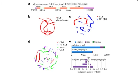
frame translations in the CCDS. We further compared results for three real datasets (ERR188040, ERR1161592, and SRR1045067) (Additional file 1: Table S2) and achieved similar results. The number of nodes and edges was approximately half that of the traditional graph, indicating that sequencing errors and false frame trans-lations increased the complexity of the codon-based de Bruijn graph. To obtain a more intuitive and compre-hensive understanding of the codon-based de Bruijn graph, the gene FBgn0039298 was taken as an example. Using all of the exons of this gene, traditional (Fig. 2a) and codon-based de Bruijn graphs (Fig. 2b) were con-structed. As shown in Fig. 2, the codon-based de Bruijn graph assembled all exons of this gene into one simple path (Fig. 2c) and exhibited considerably decreased com-plexity compared with the traditional graph (Fig. 2b). It should be noted that the codon-based de Bruijn graph also included a false CDS that did not overlap with the true CDS and thus could be easily discarded in down-stream cleaning steps. This reduced complexity was even more evident when using all elements of the gene to construct the codon-based de Bruijn graph. As shown in Fig. 2d, the graph was composed of 22 components and

most of the components contained only one path. More-over, the four exons were assembled into four separate components, each of which contained few overlaps with other elements.

The codon-based de Bruijn graph facilitates the assem-bly not only by decreasing the number of nodes and edges but also by reducing the topological complexity. To dem-onstrate this point, we used the codon-based de Bruijn graph after simplification as a benchmark. We first classified the components into three types: simple, tip-containing, and bubble-containing subgraphs. Then, the number of each type of subgraph was calculated for the graphs before and after simplification. As shown in Fig. 2e, the most dominant components in both graphs were sim-ple paths. It is important to note that even for the graph containing sequencing errors and frameshifting (Fig. 2e), 85% of the structures were simple subgraphs. Moreover, most tip-containing subgraphs had only one tip, which could easily be trimmed into simple subgraphs. Therefore, after performing graph simplification, the number of sim-ple subgraphs increased from 85% to 96%, indicating the outstanding performance of codon-based de Bruijn graphs for CDS construction and recognition.

a

b

d

c

e

Fig. 2Comparison between the traditional de Bruijn graph and the codon-based de Bruijn graph.aThe basic information of FBgn0039298 gene

inD. melanogasterused for generating the subfigures (b)–(d). The elements are marked with differentcolorsto highlight the gene structure (UTR:

purple, intron:green, exon:red).bTraditional de Bruijn graph based on simulated DNA-seq reads on CDS regions.cCodon-based de Bruijn graph

SVM filtration

To evaluate the efficiency of SVM in removing false-positive ORFs, we utilized three simulated RNA-seq datasets based on the sequences of human chr3, chr19, and chr20. First, positive and negative datasets were pre-pared to test SVM filtration. For each chromosome, the simulated reads were translated into ORFs, which were used as the test dataset. The CDSs of the chromosome were used as the positive dataset, while the sequences translated from the other five reading frames of each CDS were used as the negative dataset. Then, the sensi-tivity and specificity were calculated by aligning the predicted ORFs to the reference CDSs. As shown in Additional file 1: Figure S1A–C, SVM successfully recovered true ORFs with an average sensitivity of 90% and a specificity of 75%. We simulated four datasets with read lengths of 100, 300, 500, and 800 bp and the sensi-tivity after SVM filtration was calculated for each data-set. As shown in Fig. 3c, the sensitivity tended to improve with increasing read length. The primary factor responsible for this increase is likely to be sequence length because short sequences do not contain sufficient composition signals for discrimination.

To examine whether SVM filtration could reduce the complexity of the codon-based de Bruijn graph, we employed a real RNA-seq dataset (ERR188040) that was

first assembled by Trinity and the resulting transcripts were translated into ORFs. Two codon-based de Bruijn graphs were constructed using the translated ORFs before and after SVM filtration, and the ratio of false-positive nodes in the components of each graph was calculated (Fig. 3a). Before SVM filtration, there were a large number of false-positive nodes on the graph, which were mainly present in small components (node number <500), indicating that false-positive nodes shared few overlaps with each other or with true-positive nodes. After filtration, SVM discarded almost all of these nodes, indicating its high efficiency. Moreover, the codon-based de Bruijn graph derived from SVM-filtered ORFs exhib-ited an approximately 63% decrease in the number of components compared with the graph derived before filtration (Fig. 3b). A subset of filtered translated ORFs was taken as an example to illustrate the SVM classifica-tion result. When reducing the high dimension of SVM prediction features by principal component analysis (PCA), two distinct clusters were observed (Fig. 3d).

We also tested the impact of SVM filtration on the assembled CDSs using sequenced reads (SRR1045067). The sequenced reads were first used to predict ORFs. inGAP-CDG yielded two CDS assemblies based on the predicted ORFs with or without SVM filtration. Contig length, redundancy, average fragment number per gene,

a

c

b

d

sensitivity, and specificity of CDS recognition in the two assemblies were compared (Additional file 1: Figure S2). As expected, the CDS assembly with an SVM filtra-tion step exhibited a significantly increased CDS length compared to that without filtration (Additional file 1: Figure S2A and S2B). In addition, the CDS assembly with SVM outperformed the CDS assembly without filtration in both sensitivity and specificity (Additional file 1: Figure S2D). Therefore, we con-cluded that SVM-based filtration not only reduced the complexity of the codon-based de Bruijn graph by filtering false-positive ORFs but also improved the performance of gene recognition from fragmented sequences.

Gene prediction from assembled transcripts

Because most state-of-the-art gene prediction methods identify CDSs from assembly transcripts, we further tested the performance of inGAP-CDG on long tran-scripts. An RNA-seq dataset for human colon cancer cells (SRR1045067) was downloaded and assembled using the Trinity assembler. Both inGAP-CDG and TransDecoder were employed to predict CDSs from the resulting transcripts. As shown in Additional file 1: Figure S3A, inGAP-CDG exhibited considerably im-proved CDS length compared with TransDecoder. More-over, N50, mean, and N90 length were approximately twice as long as those from TransDecoder (Additional file 1: Figure S3B). Subsequently, the predicted CDSs were aligned with the reference gene set and matched CDSs were extracted for comparison. We found that the average length of the matched CDSs predicted by inGAP-CDG was slightly shorter than that of the refer-ence gene set, but it was significantly longer than that of TransDecoder. These nearly full-length CDSs will greatly facilitate downstream phylogenomic analyses and gene model construction. Next, the sensitivities and specific-ities of the two methods were compared and inGAP-CDG was found to exhibit higher specificity but slightly lower sensitivity (Additional file 1: Figure S3D). This decreased sensitivity is most likely due to SVM filtration, during which some true ORFs may be filtered out. Finally, we compared the redundancy of these CDSs and found that inGAP-CDS exhibited greatly decreased redundancy compared with TransDecoder (Additional file 1: Figure S3C and S3E).

Performance comparison between inGAP-CDG and 11 other strategies

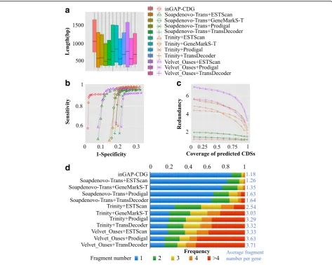
To evaluate the robustness of inGAP-CDG over different sequencing error rates, we simulated three datasets with error rates of 0.5%, 1%, and 2% and employed inGAP-CDG and 11 other pipelines to assemble and predict CDSs. The mean length, redundancy, sensitivity, and

error rate were calculated and compared. As shown in Additional file 1: Figure S4, inGAP-CDG achieved the longest mean length and the lowest redundancy among all of the approaches for all three simulated datasets. Although inGAP-CDG exhibited a moderate level of sensitivity (approximately 90%) and base error rate (0.005–0.01%), it produced the smallest fluctuation in the face of different sequencing error rates.

To demonstrate the robustness of inGAP-CDG over different read lengths, we compared inGAP-CDG with the other 11 pipelines using three real datasets (ERR188040, ERR1161592, and SRR1045067) of different read lengths (75, 100, and 150 bp). As shown in Additional file 1: Figure S5, the results varied depending on the read length. First, inGAP-CDG had the largest mean CDS length among all of the methods. Unexpect-edly, the mean CDS length decreased when the read length was increased from 75 bp to 150 bp. This decrease was observed not only for inGAP-CDG but also for the other methods and was most likely due to fact that the 150-bp reads contained more sequencing errors. Next, a comparison of sensitivity and specificity revealed that with an increase in read length, the overall sensitiv-ities and specificsensitiv-ities of all assemblies exhibited tenden-cies toward enhancement and reduction, respectively. In addition, inGAP-CDG achieved significantly higher specificity than all other methods. Notably, the specific-ities of these methods showed an increasing trend when increasing the read length from 75 bp to 150 bp. In contrast with this trend, inGAP-CDG exhibited a steady increase, demonstrating a high level of robustness for inGAP-CDG, which was achieved by discarding false translated ORFs resulting from sequencing errors and erroneous frameshifts. This robustness was also ob-served in the redundancy (Additional file 1: Figure S5C and S5D). Unlike other methods, which varied signifi-cantly when using different read lengths, inGAP-CDG exhibited only a slight fluctuation.

the predicted CDSs to this gene using the inGAP package [11, 12], different alignment profiles were observed among these methods. inGAP-CDG successfully assembled all of the reads of this gene into one CDS, and approxi-mately 100% of the gene was covered by the pre-dicted CDS. However, when using other methods, only a part of this gene was covered by the predicted CDSs and some of them included assembly chimeras. Moreover, the covered regions of this gene were aligned to multiple CDSs, a redundancy that was even more obvious in the CDSs predicted from Trinity-assembled transcripts. Similar findings were observed for the genes SET domain containing 2 (SETD, acces-sion ID: XM_011533632), dipeptidyl peptidase 7 (DPP7, accession ID: NM_013379) and acyl-CoA de-hydrogenase (ACADVL, accession ID: NM_000018),

which are all found in the NCBI database (Additional file 1: Figure S6A, C, and D). Together, these compar-isons indicate that inGAP-CDG is more reliable than other pipelines for full-length CDS prediction. We further benchmarked inGAP-CDG using three real RNA-seq datasets (SRR3332174, SRR3332175, and SRR3332176) fromD. melanogaster. After gene construction, the mean length, sensitivity, redundancy, and chimera rate of inGAP-CDG were compared with those of the other pipe-lines. Although inGAP-CDG exhibited a moderate level of sensitivity, it outperformed all other pipelines in terms of the mean length, redundancy and chimera rate for these datasets (Additional file 1: Figure S7). It should be noted that inGAP-CDG could achieve an even longer mean CDS length and lower redundancy using the strict mode, at the expense of sensitivity (4–7% decrease).

a

b

d

c

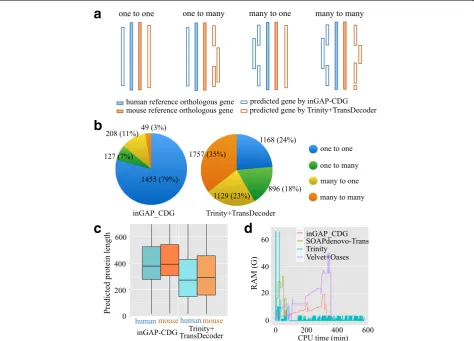
Application of inGAP-CDG to orthologous gene recognition To assess the performance of inGAP-CDG in orthology detection, we compared inGAP-CDG with a pipeline that combined Trinity with TransDecoder using two real RNA-seq datasets from H. sapiens and M. musculus brain tissues. For each dataset, the proteins were pre-dicted using these two strategies separately. After assem-bling the human dataset, inGAP-CDG yielded 14,638 ORFs with an average length of 419 codons, while the Trinity + TransDecoder pipeline produced 88,184 ORFs with an average length of 274 codons. For the mouse dataset, inGAP-CDG and the Trinity + TransDecoder pipeline generated 10,260 and 65,862 ORFs with average lengths of 481 and 304 codons, respectively. Subsequently, we retrieved the one-to-one orthologous gene pairs be-tween H. sapiensand M. musculus from the OrthoMCL database into two reference gene sets according to their original species. For each species, the predicted proteins

of these two strategies were aligned to the respective reference gene set. As a result, 3296 and 3258 proteins predicted by inGAP-CDG were aligned to the human and mouse reference gene sets, respectively, while 7219 and 7227 proteins predicted by Trinity + TransDecoder were aligned to the human and mouse reference gene sets, respectively. Finally, for each strategy, the numbers of aligned predicted proteins of two species for each paired orthologous gene were classified into four types (Fig. 5a), which represented the redundancy and completeness of each assembly and the number of predicted proteins that could be used for phylogenetic tree construction.

As shown in Fig. 5b, the most dominant type of pro-teins assembled in inGAP-CDG was one-to-one (79% of the aligned predicted proteins) and the smallest type was many, comprising only 3%. In contrast, many-to-many was the largest type in the Trinity + TransDecoder pipeline (35%), followed by one-to-one (24%), many-to-one

a

b

c

d

(23%), and one-to-many (18%). The low fluctuation among these types indicated that this pipeline produced re-dundant and incomplete genes. Moreover, inGAP-CDG outperformed this pipeline by generating more one-to-one type and fewer fragmented orthologous genes, demonstrating its predominant advantage in phylogenomic studies. We also surveyed the length distribution of aligned translated proteins (Fig. 5c) and found that inGAP-CDG exhibited an increased length compared with the combined pipeline. Such increased length will greatly facilitate the complete-ness and accuracy of phylogenetic trees.

inGAP-CDG running time and memory usage

inGAP-CDG is implemented in C++ as a standalone pro-gram. We have tested it successfully on Mac OS X EI Capitan (10.11) and Linux (Red Hat 6.3 and Ubuntu 16.04) systems. To systematically evaluate the efficiency of inGAP-CDG, the running time and RAM usage were compared with the four other gene prediction pipelines using a publicly available RNA-seq dataset (SRR1045067). Because the running time and memory usage of ESTScan, TransDecoder, Prodigal, and GeneMarkS-T were negli-gible, these tools were not included in this comparison. We ran all four programs on a node with 2.13 GHz Intel Xeon processors using eight CPUs on the Linux (Red Hat 6.3) system. As shown in Fig. 5d, among all of the pro-grams, inGAP-CDG had the lowest peak RAM, which was approximately one-third of that of Trinity. In addition, inGAP-CDG was faster than Trinity and Velvet_Oases but slower than SOAPdenovo-Trans. For the dataset SRR1045067, consisting of 4.8G bases, inGAP-CDG took approximately 350 min to construct CDSs from raw reads. In detail, six-frame translation, SVM filtration, codon-based de Bruijn graph construction, and traversal took approximately 65, 135, 120, and 30 min, respectively.

Discussion

Transcript-based gene prediction methods exhibit in-creased accuracy compared with ab initio methods, which require high-quality training datasets to ensure reliability. However, the limitations of current transcriptome assemblers have precluded these methods from generating high-quality and non-redundant CDSs. To address this challenge, we present a novel tool, inGAP-CDG, for the effective construction of full-length and non-redundant CDSs from unassembled transcriptomes. By introducing the newly developed codon-based de Bruijn graph to simplify the assembly process and SVM to filter false-posi-tives, inGAP-CDG can predict full-length CDSs at a low level of redundancy and with a low false-positive rate.

Transcriptome sequencing is an efficient and cost-effective route for generating vast sequence collections representing expressed genes. This technology provides

a valuable starting point for phylogenomic analysis in non-model organisms for which genomic sequence information is not yet available [13, 14], especially when whole-genome sequencing efforts are cost-prohibitive and time-prohibitive. Several gene recognition methods [15–17] that integrate de novo assembly and gene predic-tion have been proposed. However, these methods result in fragmented and redundant CDSs. These properties will lead to incomplete or false orthologous genes and thus generate low-quality and incongruent phylogenetic trees. However, inGAP-CDG addresses this challenge by gener-ating more one-to-one orthologous genes and improving gene completeness for phylogenomic studies.

We have demonstrated that inGAP-CDG exhibited a great advantage over all currently available transcriptome-based gene prediction methods. The primary factor underlying this advantage is the implementation of a codon-based de Bruijn graph, which contains a con-siderably decreased number of nodes and edges (by approximately 60%) compared with the traditional graph. Moreover, most of the structures in the codon-based de Bruijn graph are simple components, indicating a low level of topological complexity. Collectively, these features allow for decreased complexity and redundancy in gene prediction. Similar to the codon-based de Bruijn graph, Youngik et al. employed an amino-acid alphabet-based de Bruijn graph to simplify the traditional de Bruijn graph and reconstructed protein sequences from next-generation sequencing (NGS) metagenomic data [18]. Because each character of the amino acid alphabet-based de Bruijn graph may be one of 20 amino acids (i.e. fivefold larger than the number of nucleotides), this type of graph contains an increased number of nodes and edges while exhibiting decreased topo-logical complexity compared with the codon-based de Bruijn graph. Moreover, the outputted sequences of the amino acid alphabet-based de Bruijn graph are short peptides, which masks the original nucleic acid sequence. In addition to generating a codon-based de Bruijn graph, SVM filtration is an essential step in the inGAP-CDG algorithm. SVM discards false-positive CDSs generated by six-frame translation and yields reliable ORFs to serve as landmarks, which can dictate traversal. This filtration allows significantly increased specificity compared with other methods. Furthermore, inGAP-CDG directly recognizes CDSs from unassembled reads and consequently avoids the influence of uneven sequencing depth on assembly, which may enhance the CDS length.

result, inGAP-CDG used strict parameters in SVM to filter false-positive ORFs, which may sacrifice a small fraction of true-positive ORFs. Moreover, this filtration ensures the robustness of inGAP-CDG to sequencing errors. Further efforts could be made to improve the sensitivity of inGAP-CDG by taking into account more information (e.g. the coverage of kmers by mapping reads to the codon-based de Bruijn graph, as well as paired-end read linkage information). We believe that inGAP-CDG is an important addition to the toolbox used for phylogenomic studies and will greatly improve our capacity to explore the functional potential of novel species.

Conclusions

This study presents a novel algorithm, inGAP-CDG, for effective gene construction from unassembled transcrip-tomes. The main advantage of inGAP-CDG is that it combines a newly developed codon-based de Bruijn graph to simplify the assembly process and a machine learning based approach to filter false positives. Com-pared with traditional de Bruijn graph, the codon-based de Bruijn graph exhibits significantly decreased number of nodes and edges (by approximate 60%), as well as a considerable low level of topological complexity. These features of the codon-based de Bruijn graph allow de-creased complexity and redundancy in gene prediction. Through extensive evaluation on both simulated and real datasets, as well as comparisons with alternative methods, we demonstrate that inGAP-CDG has an excellent and unbiased performance on gene reconstruction.

Methods

Overview of inGAP-CDG

The inGAP-CDG algorithm is a four-step process that in-cludes six-frame translation, SVM filtration, codon-based de Bruijn graph construction, and traversal (Fig. 1). First, input sequences (e.g. reads or transcriptomic assemblies) are translated into potential ORFs. Due to sequencing and frame translation errors, a significant number of predicted ORFs are false positives. Next, inGAP-CDG employs a combination of SVM and codon-based de Bruijn graphing to obtain a set of highly reliable ORFs (rORFs) to serve as landmarks in the next step. Finally, because short predicted ORFs are occasionally discarded by SVM [19], inGAP-CDG builds a codon-based de Bruijn graph based on all predicted ORFs and generates full-length CDSs by traversing the graph under the guidance of rORFs (Additional file 1: Figure S8).

Codon-based de Bruijn graph construction

The input sequences are split into kmers, with a sliding window of k (default of 27 bp) and a step size of 3 bp. Then, the codon-based de Bruijn graph is built using the

resulting kmers. We define the directed de Bruijn graph as a codon-based graph G = (V, E) that has a set of verti-cesV= {v1,v2,…,vn} and a set of edges E= {(v1,v5), (v1,

v3),…, (vm,vk)|vm,vk∈V} that are formed by pairs of

k-3 bp overlapping kmers. The set of nodes is created by assigning each kmer v ∈V to a unique vertex. A path from v1 to vj through the contig graph consists of a

se-quence of nodes (e.g. (v1,v7,v4,vj)). The graph G1= (V1, E1) is a subgraph of G = (V, E) if (1) V1⊆V and (2) every edge of G1is also an edge of G. The subgraph G1= (V1, E1) is a connected component of G = (V, E) if G1satisfies three conditions: (1) V1⊆V; (2) every edge of G1is also an edge of G; and (3) any two nodes in G1are connected to each other by a path, and no paths can be found to con-nect the nodes between V1and (V–V1). A head is defined as the style of arrowhead on the head node of an edge and a tail is the style of arrowhead on the tail node of an edge.

Six-frame translation

Sequences for six-frame translation can be single-end reads, paired-end reads, or transcriptomic assemblies. If paired-end reads are provided and each pair exhibits overlaps (insert size < the summed length of a read pair), these reads are merged into long sequences using FLASH [20] software. Otherwise, these reads are treated as single-end reads. Then, for each inputted sequence, the positions of all of the stop codons are recorded. Then, all translated ORFs are collected and sorted by length. In the six-frame translation of the inGAP-CDG algorithm, we obtain two types of ORFs based on differ-ent parameters. The first type includes strict-translated ORFs that are the same length as the original sequence and do not contain a stop codon. The second type con-sists of loose-translated ORFs that cover at least 80% of the original sequence (Additional file 1: Figure S9).

SVM filtration

CDG traversal and coding sequence generation

Because some true ORFs are discarded during SVM fil-tration, a codon-based de Bruijn graph constructed from rORFs alone may result in fragmented CDSs. To solve this problem, we generated a more complete but noisy graph using the SVM test dataset (all ORFs translated via six-frame translation) and mapped rORFs to the graph to generate full-length CDSs. In detail, we split the ORFs in the test dataset into kmers and constructed a new codon-based de Bruijn graph. To simplify this graph, we executed two functions: “tips trimming” and “bubbles merging” (Additional file 1: Figure S10A–F). If a“tip,”which is defined as a chain of nodes disconnected on one end, is shorter than a given length (default: 2*kmer), it will be removed. A “bubble” is defined as several similar paths with the same start and end nodes on the graph. The paths in a bubble are compared, and the identity among these paths is calculated. If the identity reaches a cutoff of 95%, the longest path is reserved, and all other paths are discarded. The rORFs are then mapped to the simplified graph and the mapped kmers, referred to as landmarks, will be used for traversing the graph. Rather than traversing the entire graph, inGAP-CDG employs a depth-first searching algorithm, which starts at each land-mark and searches against the graph to identify the path that connects two landmarks. Once all landmarks have been visited, the nodes along the searched path are assem-bled into a final CDS. Notably, inGAP-CDG can be performed under two different modes: default and strict. The strict mode is designed to obtain longer unigenes with a lower level of redundancy. Unless specified, inGAP-CDG is performed in the default mode.

Design of simulation studies

The D. melanogaster gene FBgn0039298, downloaded

from FLYBASE [21], was used to compare the traditional and codon-based de Bruijn graphs. This gene is 5489 bp in length and contains four exons and three introns. First, a set of 100-bp single-end DNA-seq reads with a sequencing depth of 30-fold was simulated based on this gene using the Wgsim program from the SAMtools package [22] and the dataset was used by inGAP-CDG to construct a codon-based de Bruijn graph. Next, a set of 100-bp single-end RNA-seq reads was simulated from the CDSs of this gene using FluxSimulator [23] to con-struct a traditional and a codon-based de Bruijn graph.

To test the feasibility of SVM filtration, three sets of 150-bp single-end RNA-seq reads were simulated from chr3, chr19, and chr20 of the reference human genome (hg19) using FluxSimulator with the default parameters. These simulated datasets were then subjected to SVM filtration as implemented in inGAP-CDG. After SVM fil-tration, the receiver operating characteristic (ROC) curve of each dataset was plotted in R using the

LIBSVM packages (e1071). To test the effect of read length on the performance of inGAP-CDG, four RNA-seq datasets with read lengths of 100, 300, 500, and 800 were simulated from the CCDS of hg19.

To test the performance of inGAP-CDG using tran-scriptomic data with sequencing errors, three sets of 200-bp paired-end RNA-seq reads were simulated from chr3 of hg19 using RNASeqReadSimulator (https://github.-com/davidliwei/RNASeqReadSimulator) with error rates of 0.5%, 1%, and 2%, respectively. Furthermore, the metrics of sensitivity, redundancy, mean length, and base error rate were used to assess the resulting CDS predictions.

Real datasets

Three paired-end RNA-seq datasets generated from

Homo sapiens were downloaded from the NCBI

Sequence Read Archive (SRA) database [24] (accession numbers ERR188040, ERR1161592, and SRR1045067). These datasets contained 27.8, 24.4, and 19.2 million read pairs with read lengths of 75, 100, and 150 bp, re-spectively. Because the paired reads of the SRR1045067 dataset contained overlaps, we merged these reads into long reads using FLASH and obtained 13.4 million merged reads.

To verify the performance of inGAP-CDG on real data-sets, three paired-end RNA-seq datasets fromD. melano-gaster (accession numbers: SRR3332174, SRR3332175, and SRR3332176) were downloaded from the NCBI SRA database [25]. These datasets consisted of 100-bp reads and a library size of 165 bp and contained 28.9, 43.4, and 102.8 million read pairs, respectively. Because the frag-ment size of these datasets was less than twice the read length, overlapping paired-end reads were merged into long reads using FLASH to obtain 21.2, 28.5, and 81.3 million merged reads, respectively.

merged these reads into longer reads using FLASH to obtain 27.1 and 26.2 million merged reads, respectively.

Evaluation of inGAP-CDG performance

Currently, inGAP-CDG is the only tool available that can directly predict genes from unassembled transcrip-tomic reads. Several tools, such as TransDecoder (http:// transdecoder.sourceforge.net/), Prodigal [26], GenMarkS-T [27], and ESGenMarkS-TScan [28], predict genes from long tran-scripts that are generated by transcriptome assemblers (e.g. Trinity, SOAPdenovo-Trans [29], and Oases [30]). Therefore, we built several pipelines to benchmark the performance of inGAP-CDG by combining transcriptome assembly and gene prediction tools. These pipelines include: Trans + ESTScan, SOAPdenovo-Trans + GeneMarkS-T, SOAPdenovo-Trans + Prodigal, SOAPdenovo-Trans + TransDecoder, Trinity + ESTScan, Trinity + GeneMarkS-T, Trinity + Prodigal, Trinity + TransDecoder, Velvet_Oases + ESTScan, Velvet_Oases + Prodigal, and Velvet_Oases + TransDecoder. Furthermore, we prepared a reference gene set to evaluate the perform-ance of these pipelines and inGAP-CDG. We first aligned transcriptomic reads to the hg19 reference genome using TopHat [31] and used Cufflinks [32] to generate tran-scripts. The resulting transcripts were aligned to the CCDS dataset using BLAT [33] and aligned transcripts with identities greater than 95%, matched lengths longer than 1 kb and coverages greater than 90% were selected as the reference gene set.

For each pipeline and inGAP-CDG, the length distributions of the predicted CDSs were surveyed. The predicted CDSs were aligned to the reference dataset to determine the redundancy, ROC [34], aver-age fragment number per gene, base error rate, and chimera rate. Specifically, alignments with identities greater than 90%, query CDS coverages greater than 90%, and reference gene coverages greater than 90% were reserved. Redundancy was calculated as the number of aligned predicted CDSs divided by the ref-erence gene number. The ROC, which captures the trade-off between sensitivity and specificity, was deter-mined by calculating the true-positive rate (TPR) and the false-positive rate (FPR). Notably, the sensitivity is equal to the TPR, which is the percentage of the reference gene set covered by predicted genes. The specificity is 1-FPR, which represents the percentage of predicted genes covered by the reference gene set. Fragment number, which reflects the number of CDSs belonging to the same reference gene, is computed using the equation Pn_i¼1npi, where i is the number of predicted CDSs aligned to the same reference gene,n is the maximum number ofi, andpi is the prob-ability of iin all reference genes. The base error rate for a predicted CDS was calculated as the number of

mismatches divided by the alignment length. Chimeric CDSs derived from the concatenation of two or more genes were detected and the percentage of chimeras was also calculated. Specifically, the detection strategy was initi-ated with predicted CDSs larger than 500 bp and these se-quences were compared against the reference genes. A predicted CDS was treated as a chimera if it had two or more unique alignments with different genes and each align-ment accounted for at least 30% of the length of this CDS.

Moreover, we compared inGAP-CDG with the Trinty + Transdecoder pipeline for orthologous gene recognition using two real RNA-seq datasets fromH. sapiens andM. musculusbrain tissue samples. First, CDSs were predicted using these two strategies. inGAP-CDG assembled the tran-scriptomic reads according to the default parameters. In the pipeline, the reads were assembled into transcripts using Trinity with default parameters and CDSs were predicted by implementing Transdecoder on these transcripts. Next, orthologous gene pairs betweenH. sapiensandM. muscu-lus were downloaded from the OrthoMCL database [35]. The one-to-one (one human orthologous gene correspond-ing to one mouse orthologous gene) orthologous gene pairs were selected and divided into two reference datasets ac-cording to their original species. For each species, the pre-dicted proteins obtained from these two strategies were aligned to the reference dataset using BLAT. Finally, the alignments were filtered to identify mapped CDSs. In detail, alignments with identities greater than 95%, query CDS coverages greater than 50%, and reference gene coverages greater than 50% were reserved. If there was only one query CDS uniquely aligned to a reference orthologous gene, the aligned length was greater than 250 codons (i.e. half of the average reference orthologous gene length). For each one-to-one orthologous pair, the numbers of translated proteins aligned to the human and mouse reference orthologous genes were counted, respectively.

Additional file

Additional file 1:Supplementary Method.Mathematical comparison between the codon-based de Bruijn graph and the traditional de Bruijn graph.Figure S1.Efficiency of SVM on removing false positive ORFs.

Figure S2.Influence of SVM filtration on the assembled CDSs.Figure S3.

Performance of inGAP-CDG on assembled transcripts.Figure S4.Robustness of inGAP-CDG over different sequencing read errors.Figure S5.Robustness of inGAP-CDG over different read length.Figure S6.Four examples of constructed genes by inGAP-CDG and eight other pipelines.

Figure S7.Assessment of inGAP-CDG with three real RNA-seq datasets ofD. melanogaster.Figure S8.A detailed pipeline of inGAP-CDG.

Figure S9.The workflow of six-frame translation.Figure S10.Traversing the codon-based de Bruijn graph.Table S1.Comparison of the node and edge numbers between traditional de Bruijn graph and codon-based de Bruijn graph.Table S2.Datasets used in this study. (PDF 2276 kb)

Funding

Natural Science Foundation of China (91531306, 91131013), and the National Key R&D Program (2016YFC1200804).

Availability of data and materials

The inGAP-CDG software has been deposited at https://doi.org/10.5281/ zenodo.160046 and the source code is freely available at https://sourceforge.net/ projects/ingap-cdg. The software is licensed under GNU General Public License v3.

Authors’contributions

FZ proposed the method and conceived of the study. GP designed the program; GP and PJ analyzed the data. PJ, GP, and FZ wrote the manuscript. All authors discussed the results and commented on the manuscript. All authors read and approved the final manuscript.

Competing interests

The authors declare that they have no competing interests.

Ethics approval and consent to participate

This section is not applicable.

Received: 25 July 2016 Accepted: 31 October 2016

References

1. Fitch WM. Distinguishing homologous from analogous proteins. Syst Zool. 1970;19:99_–113.

2. Yang Y, Smith SA. Orthology inference in nonmodel organisms using transcriptomes and low-coverage genomes: improving accuracy and matrix occupancy for phylogenomics. Mol Biol Evol. 2014;31:3081–92.

3. Grabherr MG, Haas BJ, Yassour M, Levin JZ, Thompson DA, Amit I, et al. Full-length transcriptome assembly from RNA-Seq data without a reference genome. Nat Biotechnol. 2011;29:644–52.

4. Schweikert G, Behr J, Zien A, Zeller G, Ong CS, Sonnenburg S, et al. mGene. web: a web service for accurate computational gene finding. Nucleic Acids Res. 2009;37:W312–316.

5. Gross SS, Do CB, Sirota M, Batzoglou S. CONTRAST: a discriminative, phylogeny-free approach to multiple informant de novo gene prediction. Genome Biol. 2007;8:R269.

6. Delcher AL, Bratke KA, Powers EC, Salzberg SL. Identifying bacterial genes and endosymbiont DNA with Glimmer. Bioinformatics. 2007;23:673–9. 7. Korf I. Gene finding in novel genomes. BMC Bioinformatics. 2004;5:59. 8. Parra G, Blanco E, Guigo R. GeneID in Drosophila. Genome Res. 2000;10:511_–5. 9. Burge C, Karlin S. Prediction of complete gene structures in human

genomic DNA. J Mol Biol. 1997;268:78–94.

10. Steijger T, Abril JF, Engstrom PG, Kokocinski F, Hubbard TJ, Guigo R, et al. Assessment of transcript reconstruction methods for RNA-seq. Nat Methods. 2013;10:1177–84.

11. Qi J, Zhao F. inGAP-sv: a novel scheme to identify and visualize structural variation from paired end mapping data. Nucleic Acids Res. 2011;39:W567_–575.

12. Qi J, Zhao F, Buboltz A, Schuster SC. inGAP: an integrated next-generation genome analysis pipeline. Bioinformatics. 2010;26:127–9.

13. Chen X, Zhao X, Liu X, Warren A, Zhao F, Miao M. Phylogenomics of non-model ciliates based on transcriptomic analyses. Protein Cell. 2015;6:373_–85. 14. Ye N, Zhang X, Miao M, Fan X, Zheng Y, Xu D, et al. Saccharina genomes

provide novel insight into kelp biology. Nat Commun. 2015;6:6986. 15. Schreiber F, Pick K, Erpenbeck D, Worheide G, Morgenstern B. OrthoSelect: a

protocol for selecting orthologous groups in phylogenomics. BMC Bioinformatics. 2009;10:219.

16. Roure B, Rodriguez-Ezpeleta N, Philippe H. SCaFoS: a tool for selection, concatenation and fusion of sequences for phylogenomics. BMC Evol Biol. 2007;7 Suppl 1:S2.

17. Li H, Coghlan A, Ruan J, Coin LJ, Heriche JK, Osmotherly L, et al. TreeFam: a curated database of phylogenetic trees of animal gene families. Nucleic Acids Res. 2006;34:D572–580.

18. Yang Y, Yooseph S. SPA: a short peptide assembler for metagenomic data. Nucleic Acids Res. 2013;41:e91.

19. Chang CC, Lin CJ. LIBSVM: A Library for Support Vector Machines. ACM Trans Intell Syst Technol. 2011;2:27.

20. Magoc T, Salzberg SL. FLASH: fast length adjustment of short reads to improve genome assemblies. Bioinformatics. 2011;27:2957–63.

21. Attrill H, Falls K, Goodman JL, Millburn GH, Antonazzo G, Rey AJ, et al. FlyBase: establishing a Gene Group resource for Drosophila melanogaster. Nucleic Acids Res. 2016;44:D786–792.

22. Li H, Handsaker B, Wysoker A, Fennell T, Ruan J, Homer N, et al. The Sequence Alignment/Map format and SAMtools. Bioinformatics. 2009;25:2078_–9.

23. Griebel T, Zacher B, Ribeca P, Raineri E, Lacroix V, Guigo R, et al. Modelling and simulating generic RNA-Seq experiments with the flux simulator. Nucleic Acids Res. 2012;40:10073–83.

24. Leinonen R, Sugawara H, Shumway M. International Nucleotide Sequence Database C. The sequence read archive. Nucleic Acids Res. 2011;39:D19–21. 25. Wang Q, Taliaferro JM, Klibaite U, Hilgers V, Shaevitz JW, Rio DC. The PSI-U1 snRNP interaction regulates male mating behavior in Drosophila. Proc Natl Acad Sci U S A. 2016;113:5269_–74.

26. Hyatt D, Chen GL, Locascio PF, Land ML, Larimer FW, Hauser LJ. Prodigal: prokaryotic gene recognition and translation initiation site identification. BMC Bioinformatics. 2010;11:119.

27. Tang S, Lomsadze A, Borodovsky M. Identification of protein coding regions in RNA transcripts. Nucleic Acids Res. 2015;43:e78.

28. Iseli C, Jongeneel CV, Bucher P. ESTScan: a program for detecting, evaluating, and reconstructing potential coding regions in EST sequences. Proc Int Conf Intell Syst Mol Biol. 1999:138_–48. https://www.ncbi.nlm.nih. gov/pubmed/10786296.

29. Xie Y, Wu G, Tang J, Luo R, Patterson J, Liu S, et al. SOAPdenovo-Trans: de novo transcriptome assembly with short RNA-Seq reads. Bioinformatics. 2014;30:1660_–6.

30. Schulz MH, Zerbino DR, Vingron M, Birney E. Oases: robust de novo RNA-seq assembly across the dynamic range of expression levels. Bioinformatics. 2012;28:1086–92.

31. Trapnell C, Pachter L, Salzberg SL. TopHat: discovering splice junctions with RNA-Seq. Bioinformatics. 2009;25:1105–11.

32. Trapnell C, Roberts A, Goff L, Pertea G, Kim D, Kelley DR, et al. Differential gene and transcript expression analysis of RNA-seq experiments with TopHat and Cufflinks. Nat Protoc. 2012;7:562_–78.

33. Kent WJ. BLAT–the BLAST-like alignment tool. Genome Res. 2002;12:656–64. 34. Sing T, Sander O, Beerenwinkel N, Lengauer T. ROCR: visualizing classifier

performance in R. Bioinformatics. 2005;21:3940–1.

35. Chen F, Mackey AJ, Stoeckert Jr CJ, Roos DS. OrthoMCL-DB: querying a comprehensive multi-species collection of ortholog groups. Nucleic Acids Res. 2006;34:D363–368.

• We accept pre-submission inquiries

• Our selector tool helps you to find the most relevant journal

• We provide round the clock customer support

• Convenient online submission

• Thorough peer review

• Inclusion in PubMed and all major indexing services

• Maximum visibility for your research

Submit your manuscript at www.biomedcentral.com/submit