Short Term Load Forecasting Using Moving Averages

Technology (IJRASET)

Short Term Load Forecasting Using Moving

Averages

Mr. Sandeep Tiwari1, Mr. Kamlesh Lahre2

1

M. Tech Student Dept.of CSE CVRU Bilaspur, 2Asst.Professor, Dept. of CSE CVRU Bilaspur

Abstract: Electricity is an essential part of our life and without this nothing is possible an accurate and efficient Short term load forecasting plays a vital role for economic operational planning of both regulated power systems and electricity markets. Short term forecasting including energy purchasing and generation, infrastructure development and load switching . A large variety of mathematical methods have been developed for load forecasting. This paper proposed the multiplicative decomposition model and the smoothing techniques model. Forecasting errors of both models are computed and compared. Results show that both time series models can accurately predict the short-term demand.

Keywords— Short Term load forecasting, moving averages, exponential smoothing, mean Absolute Percentage Error (MAPE)

I. INTRODUCTION

The short-term load forecast is of importance in the daily operations of a power utility. It is required for unit commitment, energy transfer scheduling and load dispatch. With the emergence of load management strategies, the short-term load forecast has played a broader role in utility operations. The development of an accurate, fast and robust short-term load forecasting methodology is of importance to both the electric utility and its customers. Several different methods, techniques and algorithm have been developed to forecast load demands, with the focus on improving the prediction accuracy. The approach using time series analysis is among the main areas with rich research effort, with specially formulated methods for data in various contexts. Two time series models, namely, the multiplicative decomposition model and the smoothing techniques model employed. The multiplicative decomposition technique has been profoundly used for forecasting tasks in the business sector, such as sales projection or financial forecasting. However, it has not been commonly employed for electricity demand forecasting. This may due to the fact that load demands usually vary to a large extent across seasons with changing temperatures and it is challenging to fit a trend line. Thus, this technique is proposed in this paper. The proposed models are implemented to predict one week demand data. The accuracy of the two models are calculated and compared. The paper utilizes the mean absolute percentage error (MAPE) as a measure of forecast accuracy. The paper is organized as follows. Section II introduces the two above mentioned models and explains how they would be used in analysing and forecasting the load consumption with a brief note on forecasting error measurement. Section III is the case study where by demands are first plotted for visual comparison of weekday and weekend data. Then models would be applied with forecasts generated and compared with the amounts actually consumed.

II. TIMESERIESMODELS

Time series is defined as a set of data generated sequentially in time. The time series models assume that in the absence of major disruptions to critical factors of a recurring event, the data of this event in the future will be related to that of the past events and can be expressed via models developed from the past events. In this analysis, two time series models, the Multiplicative Decomposition Model and the smoothing techniques. Model are employed and presented in the followings.

A. Multiplicative decomposition model

Technology (IJRASET)

remove the seasonal component from the series. To find the indexes, data of the most recent week without any holiday are divided by the average of a few recent weeks and using the average of these weeks tends to minimize the random effect. With these two components removed or minimized, the series now contains mainly the trend component. The equation of this trend line is extrapolated to estimate the trend in the future. Seasonal effects can then be incorporated into these future trend forecasts to account for the intra-day variation and obtain reasonably comprehensive forecasts. In the following, the detail implementation is described.

1) Intraday Seasonal Index: This section analyses intra-day seasonal index which measures how the series evolve throughout a day in order to predict future load performance on a half-hourly basis. Due to distinct difference of the data between weekend and weekday in terms of magnitude and fluctuation, weekends will be taken off the series and analysed separately from weekdays. First, the average of all measurements from the immediately previous four weeks (weekdays) is calculated. The rational for choosing a four-week period is to reduce the effect of the possible scenario that a holiday exists within the past week and distorts the weekly seasonal behaviour. In addition, data in the past weeks may not reflect the current situation well therefore only the latest four weeks are chosen. Next, each of the latest week’s data is divided by the four-week average to give the weekly seasonal indexes. If a holiday is present in the latest week, the previous week is used instead to represent a typical weekly performance. The weekly seasonal indexes represent how each half-hourly measurement varies across the week and typically range from 80% to 120% of the four-week average.

2) Depersonalized Weekly Trend:A depersonalized weekly performance is obtained by dividing the latest week’s data (or the previous week’s, whichever is used) by the weekly seasonal indexes correspondingly. This is the depersonalized weekly trend which is expected to appear as a straight trend line with small variations due to random effects that we cannot remove completely.

3) Forecasting: Equation to the weekly trend can be easily obtained by mathematical derivation or software tools, such as MATLAB or WEKA. This will then be used to project into the future for future trend in a process called trend forecasting. The actual forecast is done by multiplying this forecasted trend with the weekly seasonal indexes. This process can be extended from a single week to two weeks or more. However, it should be noted that the past data is related more closely to the immediate next week and that the forecast tends to have more significant errors for data points further into the future. This is due to many unforeseen factors which are difficult to simulate accurately. When a holiday is anticipated in the forecasted duration, great care must be taken to consider that particular day’s forecast to be similar to its form in the last occurrence. No universal seasonal indexes are possible for all holidays because during different holidays, the system load dynamics behave differently. For example, Chinese New Year holidays usually see a major drop in demand magnitude for two days while other single public holidays have lower demands only on that particular day. These holidays seem to resemble to a certain extent a typical Sunday’s load curve but even more closely, the curve of the correspondingly holidays one year ago. In this analysis, previous year’s holiday data is mapped into the forecasted year, with the magnitude appropriately adjusted for development in the year. After the forecast is done for weekdays, we will forecast for weekends data in a similar manner. Combining these two forecasts will give us the overall forecast of the future load.

III.MULTIPLICATIVEDECOMPOSITIONMODEL

Technology (IJRASET)

Fig:1 Depersonalized Load in hours

Multiplying them with the weekly seasonal indexes will give the final forecasts. Weekends are similarly analyzed and forecasted. Afterwards forecasts are joined together as overall forecasts for the entire month.

Fig:2 Forecast and Actual Load Comparison

A. Smoothing Techniques

1) Introduction To Smoothing Techniques: Smoothing techniques are used to reduce irregularities (random fluctuations) in time series data. They provide a clearer view of the true underlying behaviour of the series. Moving averages rank among the most popular techniques for the pre-processing of time series. They are used to filter random "white noise" from the data, to make the time series smoother or even to emphasize certain informational components contained in the time series.

2) Different Smoothing Techniques: Many Smoothing Techniques are there but Moving Averages is the popular technique to smooth the data. So we are explaining the Moving Average Techniques below, Moving Averages: A moving average (MA) is an average of data for a certain number of time periods. It "moves" because for each calculation, we use the latest x number of time periods' data. Using an average of prices, moving averages smooth a data series and make it easier to spot trends. This can be especially helpful in volatile markets. Types of Moving Average: There are three major types of Moving Averages: Simple Moving average, Expontional Moving average and weighted moving average.

Technology (IJRASET)

drops the first data point (11) and adds the new data point (16). The third day of the moving average continues by dropping the first data point (12) and adding the new data point (17). Notice that the moving average also rises from 13 to 15 over a three day calculation period. Also notice that each moving average value is just below the last price. For example, the moving average for day one equals 13 and the last price is 15. Prices the prior four days were lower and this causes the moving average to lag

4) Exponential Moving Averages (EMA): Exponential moving averages reduce the lag by applying more weight to recent prices. The weighting applied to the most recent price depends on the number of periods in the moving average. An exponential moving average is similar to a simple moving average, but whereas a simple moving average removes the oldest prices as new prices become available, an exponential moving average calculates the average of all historical ranges, starting at the point you specify. There are three steps to calculating an exponential moving average. First, calculate the simple moving average. An exponential moving average (EMA) has to start somewhere so a simple moving average is used as the previous period's EMA in the first calculation. Second, calculate the weighting multiplier. Third, calculate the exponential moving average. The formula below is for a 10-day EMA.

SMA: 10 period sum / 10

Multiplier: (2 / (Time periods + 1))= (2 / (10 + 1))= 0.1818 (18.18%) EMA: {Close–SMA (previous day)} x multiplier + EMA (previous day). Or we can also write this formula like (SMA +multiplier (Last value–SMA)

5) Weighted Moving Average (WMA): This average is calculated by multiplying each of the previous day’s data by weight. Therefore it is designed to put more weight on recent data and less weight on past data. In other words, it is simply a moving average that is weighted so that more recent values are more heavily weighted than values further in the past. Evidence also indicates that the use of this type of moving average gives better volatility estimates than the simple moving average. The formula of the WMA averageis:1)) * Pn-(n-1)) / (n + (n-1) + ... + (n-(n-1))) W ((n * Pn) + ((n - 1) * Pn-1) + ((n - 2) * Pn-2) + ... ((n - (n – 1))) here n is the number of terms present, p is the values given there. The WMA of prices of 1.2900, 1.2900, 1.2903, and 1.2904 would give a moving average of 1.2903 using the calculation ((4 * 1.2904) + (3 * 1.2903) + (2 * 1.2900) + (1 * 1.2900)) / (4 + 3 + 2+ 1) = 1.2903

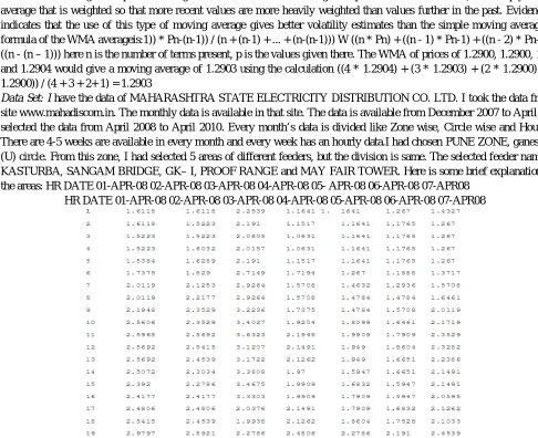
6) Data Set: I have the data of MAHARASHTRA STATE ELECTRICITY DISTRIBUTION CO. LTD. I took the data from the site www.mahadiscom.in. The monthly data is available in that site. The data is available from December 2007 to April 2010 I selected the data from April 2008 to April 2010. Every month’s data is divided like Zone wise, Circle wise and Hour wise. There are 4-5 weeks are available in every month and every week has an hourly data.I had chosen PUNE ZONE, ganeshkhind (U) circle. From this zone, I had selected 5 areas of different feeders, but the division is same. The selected feeder names are: KASTURBA, SANGAM BRIDGE, GK– I, PROOF RANGE and MAY FAIR TOWER. Here is some brief explanation of all the areas: HR DATE 01-APR-08 02-APR-08 03-APR-08 04-APR-08 05- APR-08 06-APR-08 07-APR08

HR DATE 01-APR-08 02-APR-08 03-APR-08 04-APR-08 05-APR-08 06-APR-08 07-APR08

Technology (IJRASET)

This is the weekly data with 24 hours each, Like that I have a data of 2 years that is from April 2008 to April 2010 of 5 areas. The three variables of the data are: HR–hour Date Day–Monday to Sunday

I used this data for the predictive analysis. Using the different smoothing techniques on the data, I had predicted the future values, their load and I also calculate their accuracy as well

7) Simple Moving Average: we can calculate the SMA and steeps to perform the SMA on our data set. How Pre-process the raw data, also learn to use MS-Excel for Time Series Analysis.

B. Introduction to Simple Moving Average

The moving average which serves as an estimate of the next period value of a variable given a period of length “n”. For example, a 10-day simple moving average of closing price is the mean of the previous 10 days' closing prices. If those prices are then the formula is

1) Steps Use to Calculate The Sma

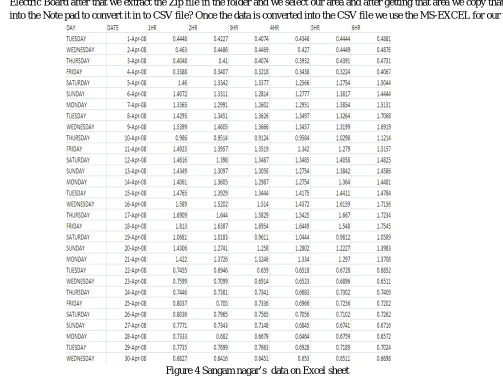
a) Step 1: We down load the raw data from the web site www.mahadiscom.in. Which is an official web site of the Maharashtra Electric Board after that we extract the Zip file in the folder and we select our area and after getting that area we copy that data into the Note pad to convert it in to CSV file? Once the data is converted into the CSV file we use the MS-EXCEL for our work.

Figure 4 Sangam nagar’s data on Excel sheet

Technology (IJRASET)

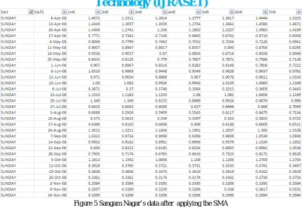
Figure 5 Sangam Nagar’s data after applying the SMA

c) Step 3: SMA is Average value so we are using the simple formula to calculate the SMA the formula is SMA= sum of number of values / N, where N is the total numbers of values present in the sample. We are using the same formula to calculate the SMA in our data set.

Technology (IJRASET)

the data like 3PSMA, 4PSMA, 5PSMA, 6PSMA.7PSMA. Results are constant so up to 7PSMA. Therefore no need to use more periods.

d) Step 4: In our data set we have calculated the 3PSMA, 4PSMA, 5PSMA, 6PSMA, 7PSMA to predict the load of upcoming Sunday. We are taking the data from our data set to solve these calculations. To calculate the 3PSMA we need three values so we are taking three values from our data set these values are 1.6041, 1.5199, and 1.475

3PSMA = (N1+N2+N3)/N 3PSMA = (1.6041+1.5199+1.475)/3

3PSMA=1.533 For 4PSMA we take four values from our data set like 1.6041, 1.5199, 1.475 and 0.769 and apply the formula 4PSMA=(N1+N2+N3+N4)/N

4PSMA = (1.6041+1.5199+1.475+0.769)/4 4PSMA=1.342 Like this I apply this formula up to 7PSMA in our data set.

e) Result

Actual Value Predicted Values

Figure 7 Calculated values of SMA.

This is the result of the 1st hour data, after applying SMA. We got one actual value and five predicted values SUM= It is the additions of the total numbers of values present on the data set.

MEAN =Sum of vales / Total number

MAPE=Mean absolute percentage error is measure of accuracy in a fitted time series.

Where At is the actual value and Ft is the forecast value.

ACTUAL VALUE= It the original value, here the Actual value is 77.7605

PREDICATED VALUE = It is the calculated value here the Predicated value is 75.10573, 73.829, 72.56248, 71.45563, 70.372. ACCURACY= It is a measurement of a correctness; the accuracy of the model is near about 97%. ACCURACY = MAPE*100

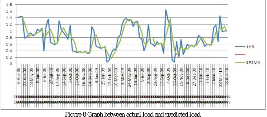
Figure 8 Graph between actual load and predicted load.

Technology (IJRASET)

denotes the Actual data and Light Green line denotes the 3PSMA. In this way, we can calculate Simple Moving Average for all 24 hours.

C. How To Calculate The Predicted Values

We need to calculate the simple moving average of the data. Then we need to calculate the accuracy of all the models 3PSMA gives us the Accuracy up to 97% so we are using the 3PSMA to calculate the load for the upcoming day.

For calculating the predicted values, we can select the last three values of 3PSMA of the 1st hour. We can calculate the 3PSMA of last three values

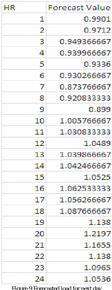
Ex 0.9709+0.9997+0.9997/ 3 = 0.9901.

It is the predicted value of 1st hour. For predicting 2nd, 3rd up to 24th hour value, we can use 3PSMAtechnique on the last three values.

Technology (IJRASET)

Figure 10 Graphical representation of forecasted load.

This is the graph, which shows the load of the predicted values of all the 24 hours, after using the SMA technique.

REFERENCES

[1] I.H. Witten and E. Frank, Data Mining Practical Machine Learning Tools and Techniques Second edition Morgan Kaufmann, San Francisco, CA, 2005. [2] J. Han and M. Kamber, “Data Mining Concepts and Techniques” Second edition, Morgan Kaufmann, San Francisco, CA 94111, 2005

[3] J. Shafer, R. Agrawal, and M. Mehta. SPRINT : A scalable parallel classifier for data mining. VLDB’96

[4] K. Liu, S. Subbarayan, R. R. Shoults, M. T. Manry, C. Kwan, F. L. Lewis and J. Naccarino, "Comparison of very short-term load forecasting techniques," IEEE Trans. PowerSyst., Vol. 11, No. 2, May 2002. http://archive.ics.uci.edu/ml/datasets.html

[5] L. Kaufman and P. J. Rousseeuw. Finding Groups in Data: an Introduction to Cluster Analysis. John Wiley & Sons, 1990 [6] objhyndman.com/researchtips/forecasting-and-time-series-books

[7] M. S. Bartlett. “On the Theoretical Specification of Sampling Properties of Autocorrelated Time Series.” Journal of the Royal Statistical Society, B8, 27 (1946).

[8] http://archive.ics.uci.edu/ml/datasets/Auto+MPG [9] Weka 3.6.3 …. Data set

[10] http://www.mahadiscom.in/

[11] http://www.mahadiscom.in/