Effective Power Consumption Model for the Network
Coded Smart Senor Network
Rachna Tewani
Faculty of Engg & Tech. MRIUFaridabad,India
D.S Gotra
Associate Director,FET MRIU Faridabad,India
ABSTRACT
A realistic power consumption model of wireless communication subsystems typically used in many sensor network node devices is presented. The sensor network facilitates monitoring and controlling of physical environments. These wireless networks consist of dense collection of sensors capable of collection and dissemination of data. They have application in a variety of fields such as military purposes, environment monitoring etc. Typical deployment of sensor network assumes the central processing station or a gateway to which all other nodes for routing data from source to sink using sensor protocol for information via negotiation protocol. Continually sending the data from the natural environment which is necessary needed causes congestion at central station and thus reduces the efficiency of the network results low power life. In this work we will propose a better Sensor Protocol For Information Via Negotiation routing technique using network coding to reduce the total number of transmission and reception in sensor networks resulting in better efficiency as well as power consumption. This power consumption model can be used to guide design choices at many different layers of the design space including, topology design, node placement, energy efficient routing schemes, power management and the hardware design of future wireless sensor network devices.
Keywords
Sensor Protocol For Information Via Negotiation, Network Coding, Wireless Sensor Network.
1. INTRODUCTION
Wireless sensor networks (WSNs) are one of the most popular networks used in computer science. It consists of some autonomous sensors used to monitor various natural activities. These natural activities may be pressure, temperature, sound vibration etc.. Sensor nodes collect data from natural activities and pass it to a central processing station or gateway called sink [1]. Lots of research has been made in various areas to enhance the overall throughput of WSNs. Development of WSNs actuated by some important applications like military surveillance’s, medical sciences, natural disaster control, etc. The topology of WSNs consists of multiple sources and single sink. This causes some common problems like congestion at the sink, limited resources, limited battery life of sensor nodes etc. Because of limited resources inefficient routing is also a major problem for WSNs. Efficient Sensor Protocol For Information Via Negotiation routing helps to increase the overall throughput of the WSNs.
1.1 Sensor Protocol for Information via
Negotiation (SPIN) & AODV
SPIN (Sensor Protocols for Information via Negotiation) efficiently disseminates information among sensors in an energy constrained wireless sensor network. Nodes running a SPIN communication protocol name their data using high level data descriptors, called metadata. They use metadata
negotiations to eliminate the transmission of redundant data throughout the network. In addition, SPIN nodes can base their communication decisions both upon application specific knowledge of the data and upon knowledge of the resources that are available to them. This allows the sensors to efficiently distribute data given a limited energy supply. SPIN protocols can deliver 60% more data for a given amount of energy than conventional approaches. We also find that, in terms of dissemination rate and energy usage, the SPIN protocols perform close to the theoretical optimum.
SPIN nodes use three types of messages to communicate:
ADV (new data advertisement) When a SPIN node has data to share, it can advertise this fact by transmitting an ADV message containing metadata.
REQ (request for data) -A SPIN node sends a REQ message when it wishes to receive some actual data.
DATA (data message) - DATA messages contain actual sensor data with a metadata header [16] [17].
Ad hoc On-demand Distance Vec- tor (AODV) [11] is a reactive routing protocol therefore routes are determined when needed.
1.2 Network Coding
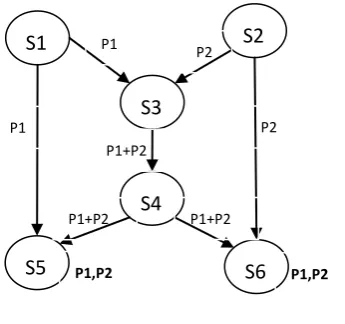
Network coding is the technique which is extensively used in wired networks, ad-hoc networks, and distributed sensor networks, etc. Network coding is quite different from traditional communication. Network coding achieves vast performance gains by permitting intermediate nodes to carry out algebraic operations on the incoming data [10]. Network coding allows the packets to encode and further forward it. The destination sink decodes the packets. Encoding is simply XOR of data packets which will be called as encoded packet. XOR is simply exclusive-or of the packets can easily be obtained from an XOR truth table. Suppose node Px and Py are two packets. Such that Px=10110 and Py=01101. Packet encoding=Px XOR Py=10110 XOR 01101= 11011=Pz. Packet decoding=Px XOR Pz=10110 XOR 11011=01101=Py and Py XOR Pz=01101 XOR 11011=10110=Px. Where Pz is encoded packet. Decoding is the XOR of data packets (except the missing one) and the encoded packet as a result the missing packet gets identified [2], [9], [10].
Consider a sensor network in Figure 1 having six nodes. Node S1, S2, S3, S4, S5 & S6 has some packet data to share with each and every node. Assume all links have a time unit capacity. In the current approach, S1 and S2 transmissions their data and was listened by their neigh boring node according to Figure 1. Now there is a bottleneck on node S3 2 data packets for transmission. Node S3 both the 4 data packets one by one. Each node listens these transmissions and collects their data packet. This approach requires 6 transmissions in all.
20 and have an opportunity of encoding the packets. Node S3
encode the data packets and transmits. Finally received by S5 and S6. Both the nodes decode the data packets as discussed earlier. By going this way only 4 transmissions is required. Now this approach requires 4 transmissions which are 37 % less than previously discussed approach. This also reduces the bottleneck, congestion at the sink and total transmission on the network and in the process provides gain in bandwidth, efficiency and power resources of the nodes [14].
Figure 1: Network Coding
1.3 Power consumption model for MultiHop
WSN:
In this section, we derive a power consumption model for the communication subsystem of a wireless sensor network device. In this model, the physical communication rate is constant and assumed to be B bits per second. In addition, we initially assume the communication bandwidth is low enough that interference and transmission collisions can be easily avoided by using simple protocols without significant power consumption penalty.
In order to evaluate the power consumption model for a multihop network, a network model is needed. If we assume a channel model, which only includes path loss then a multi-hop routing scheme will perform the best in a simple 1-D linear WSN topology. The single-hop 1-D linear WSN consists of a source node S and a destination node D separated by a distance R, and multi-hop 1-D linear WSN has an additional n-1 intermediate identical relay nodes Ni, i=1, …n-1, placed in a line from S to D (see Figure 2). In Figure 3(b), the relay nodes are placed an arbitrary distance apart, and in Figure 2(c) the relay nodes are placed equidistantly. The objective of the WSN is the reliable delivery of the data generated at the source node to the destination node.
[image:2.595.325.535.78.244.2]PR describes the power consumption for receiving. PT(di) denotes the power consumption for transmitting over a distance d. i is an integer from 1 to the total number of hops, n. PT(R/n) denotes power consumption for transmitting over a distance R/n. We use P(n) to denote the total power consumption for sending from S to D with n-hops. We ignore the power consumption in the destination node D, because it is assumed to be connected to an external power supply and is not resourced constrained. Based on the network model in Figure 2(b) and equations, we can obtain the multi-hop power consumption model with arbitrary distance between nodes as follows:
Figure 2: Network Model
\
Similarly, based on the network model in Figure 2 2(c), we can obtain the multi-hop power consumption model with equal distance between nodes as follows:
In particular, this model of WSN power consumption clearly shows the dependence of the power amplifier performance (i.e. drain efficiency, η), which differs from other power consumption models widely cited by the WSN research community [15].
1.4 Deployment strategy for WSNs
Efficient deployment strategy is necessary to detect event occur in WSNs and obtain the real time data. For example of a large dense forest there no need deploy WSNs in mountain region. This can be done by deploying sub sensor networks in a distributed manner. Density of sensors depends on the occurrence of events. The positions of sensors are predetermined and position of sensor nodes identified by GPS systems. Each transmission contains a source ID and Sink ID and transmission is directed to sink node [4], [7]. Proposed topology can be viewed as subsequent part of large sensor network where each node taking part in data transmission using current communication approaches.
2 RELATED WORK
The wireless sensor node, being a microelectronic device, can only be equipped with a limited power source (< 0.5 Ah, 1.2 V). In some application scenarios, replenishment of power resources might be impossible. Sensor node lifetime, therefore, shows a strong dependence on battery lifetime. In a multi-hop ad hoc sensor network, each node plays the dual role of data originator and data router. The malfunctioning of a few nodes can cause significant topological changes and might require rerouting of packets and reorganization of the network. Hence, power conservation and power management take on additional importance. It is for these reasons that researchers are currently focusing on the design of poweraware protocols and algorithms for sensor networks. In this section we explore the history of network coding and wireless sensor protocol for information via negotiation routing (SPIN). Our major concentration of the work is to concentrate on overall power consumption of the wireless sensor networks. Ahlswede et al. [1] showed that with network coding, as symbol size approaches infinity, a source can multicast information at a rate approaching the smallest minimum cut between the source and any receiver. Practical
S3
S1
S2
S6
S4
S5
P1
P1 P2
P2 P1+P2
P1+P2 P1+P2
[image:2.595.99.272.165.327.2]deployment of network coding is thoroughly described in [5], [7], [8].Various network coding techniques like linear and random network coding are classified in [9]. [6] Provides a systematic method to quantify the benefits of using network coding in the presence of multiple concurrent unicast sessions. A robust network coding aware data aggregation approach which will result in better performance of the network by reducing the number of transmitting messages in the network is discussed in [4]. It also gives protection from link failure to many-to-many network flows from multiple sensor nodes to sink nodes. Benefits of network coding over wireless networks are described in [14]. Various efficient sensor protocols for information via negotiation routing (SPIN) techniques are explained in [3], [12], [13]. Also large WSNs topologies are described in [4]. This gives us motivation to implement better sensor protocol for information via negotiation routing (SPIN) for large WSNs using network coding.
3 PROPOSED SCHEME
In this section we will discuss system model, proposed approach and algorithms for the proposed scheme.
3.1 Proposed System Model
In this work we have assumed the sensor node transmitting the data are aligned in a systematic manner along with specific topology. The sensor node collects the data from the environment (i.e. temperature, pressure, vibration etc..) and transmits in the direction of sink nodes by using intermediate nodes. Sink node collects the proper data and transmits of base station where the data can be processed. In this work we have classified the nodes in 3 categories. One is sensor nodes who collect data nodes and transmits, the other is a relay node whose only work is to forward the data towards the direction of sink node, third one is aggregate node in which our network coding algorithm is implemented namely aggregate node. Aggregate node finds out the network ending opportunity by using the proposed algorithm which we will discuss later and transmits encoded data to relay node. Topology of the sensor network can be deployed by referring to the figure. Topology is recursive and scale up to infinity. Topology can be constructed recursively with Level L1, Level L2, Level L3 ---Level N Level L0 is always constant and containing 5 relay nodes and a single node. Now level L1 contains R+G nodes R is of sensor nodes and G is of aggregate nodes No of aggregate nodes always half of the No of sensor nodes Bow basic topology constructed by making L0+L1.
Now level L2 can be constructed as 2(R+G) node or 2L1 nodes. By this way as scalable topology can be constructed by making L0+L1+L2………Ln. This recursive method continues and helps to construct a scale able sensor network. Figure have level L1 topology.
To better result are making some assumptions:
• Two dimensional node topology
• Each sensor node has its unique Id and single node maintains the Id of these sensor nodes.
• Each adjacent node must approx. in equal distance. • Nodes must approximately at equal distance. • Let P & G are two received data packets by the
aggregate nodes and binomial f which of computes the significant difference between the two data values and return 0 or 1 if p & q are differs more than γ then the value of the function returns 0 else remains 1. The absolute value of the difference is denoted by d = p ~ q. ƒ :{ 0 if d < γ, 1 else}
3.2 Proposed Work
In this work we would give attention on basic design and power consumption sensor network to overall throughput focus of our work is basically on the best placement of sensor nodes as well as to achieve better power consumption for the overall sensor networks.
By implementing network coding technique at the aggregate nodes and decoding at the sink as algorithms discussed in the next section. We have achieved a reduction in the total number of transmission as well as the total of the reception of data packets on the intermediate nodes from source sink, In this paper we have used constraint topology to achieve much better result in overall power consumption of the nodes.
Node placement is in two dimensional as shown in Fig 2. Now node {1} is sink node. Nodes {5, 6, 8, and 9} are aggregate nodes. Nodes {2, 3, 4, 7, and 10} are relay nodes. Nodes {11, 12, 13, 14, 15, 16, 17 and 18} are sensor nodes.
For Example supposes sensor node 12 and 13 have some information to write. Now node 12 forwards (Transmissions) its information to relay node 10 and aggregate node 9 and sensor node 13 forwards its information to aggregate node 9. Relay node simply forwards its information to sink node. Aggregate node 9 has two packets to forward. It encodes the packets using (XOR) technique and further forwards it to sink. Now sink has two packets. One is a data packet transmitted by node 12 via relay node 10 and encoded packet transmitted by aggregate node 9. It simply decodes the packet by again XORing both the packets and collect the data packet transmitted by sensor node 13. Here we can clearly see that sink node achieves the packets in 6 transmissions instead of 8 which is currently done by AODV.
Before hopping to algorithm 1 would like to put emphasis upon the point that we are not providing the answer to the question: "When to encode data?”. For the purpose of this work we have used a random variable to decide upon when to encode, with equal probabilities.
3.3
Algorithms
To enable encoding and decoding of packets we have used two types of packets namely normal_packet and code_packet. Where size of normal_packet is fixed and size of code_packet is will be size of normal_packet plus the size of the header.
Let at an aggregator node we need to encode pkt1 and pkt2. This is done as follows: pkt1 is XORed with pkt2 and is encapsulated under new header and is then forwarded depending upon the new header. We have also included a bit in each packet namely codeOn bit which is set if packet is code_packet and unset if it is normal_packet (though it is redundant as type of packet can be identified by size) in our case. Decoding is performed by first removing the additional header and then again XORing the packet with other appropriate packets.
3.3.1 Packet encoding
22
Figure 3: Sensor network topology
Algorithm: Packet_encode(packet pkt1, packet pkt2) //pkt1i& pkt2i is ith packet sent by leaf node 1 and leaf node 2 respectively.
{
Apply function f on data(pkt1i), data(pkt2i) and if it returns 0 then
{
If data(pkt1i),data(pkt1i-1) not equals to 0 then
{
Perform network coding on pkt1i and pkt1i-1 // pkt1i-1 is cached copy
Transmit data obtained by encoding in the previous step }
ElseIf data(pkt2i),data(pkt2i-1) not equals 0 {
Perform network coding on pkt2i and pkt2i-1
Transmit data obtained by encoding in the previous step }
Else
{
Select either of the packet and transmit }
}
Else
{
Perform network coding on pkt1 and pkt2
Transmit data obtained by encoding in the previous step }
//End of Algorithm Function data(packet pkt) {
Return data encapsulated in packet "pkt" }
Algo1: Algorithm for aggregate node
3.3.2 Packet Decoding:
Packet decoding is simple. Each node maintains a Packet Pool, having a copy of each neighbour packet it has received or sent. Each packet is stored in a hash table keyed on packet id, and the table is garbage collected every few seconds. When a sink node receives an encoded packet consisting of n native packets, the node goes through the ids of the native packets one by one, and decodes the corresponding packet from its packet pool if possible. Ultimately, it XORs the n−1 packets with the received encoded packet to retrieve the native packet meant for it.
4 SIMULATION RESULTS
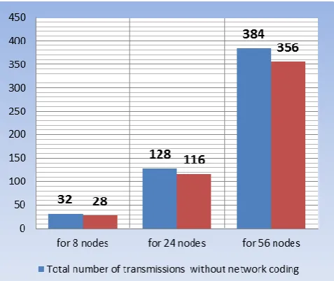
Given algorithm is implemented in Matlab R2010a & NS2. Traffic is generated using a CBR traffic generator at leaf nodes. We have simulated the discussed algorithm on topologies of 8, 24 and 56 nodes. AS mentioned earlier, function ƒ is simulated with the help of random variables. Caching is only implemented at aggregate node with cache buffer size of two, one for each leaf node. Results of simulations are given in Figure 4, Figure 5 & Figure 6 for both types of network that is to say the network without coding and network with coding. Each simulation is run four times and so each bar represents average of four simulation runs. This is done to mitigate the effect of random variable and simulation parameters.
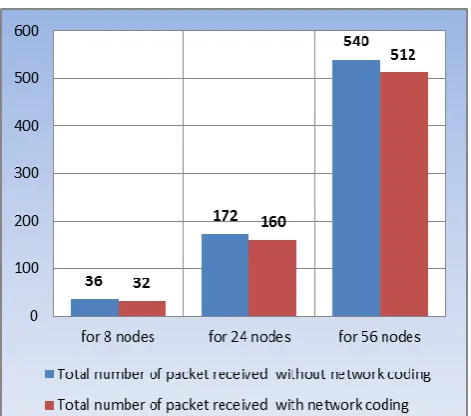
[image:4.595.61.278.73.361.2]Figure 4 clearly states the total no packet transmissions with and without network coding. One can clearly see that total no of packet transmission with network coding is slightly less than the total number of packet transmission without network coding. Similarly Figure 5 clearly states the total no packet received with and without network coding. One can clearly see that total no of packet received with network coding is slightly less than the total number of packets received without network coding. Figure 6 states the variation in overall power consumption with and without network coding.
Figure 4: Simulation results (Packet transmitted)
15
Wireless Link 1
2 3
4
5
6
7
8
9 10
11
12
13 16
17
18
Sink Node
Relay Node
Aggregate Node
Sensor Node
[image:4.595.49.284.375.715.2] [image:4.595.316.555.451.652.2]23
Figure 5: Simulation results (Packets Received)
[image:5.595.55.288.323.535.2]
Figure 6: Simulation Results (Power consumption (mW))
5 CONCLUSIONS AND FUTURE WORK
In this paper we have implemented the idea presented in [15] and [16]. We have found out that as the size of sensor network increases, approach with network coding allows better power consumption utilization. Though we have not quantified, one could easily argue, as number of transmissions required to send one packet from leaf node to sink nodes decrease it also provides significant energy savings at sensor nodes. Although the topology suggested is scalable and robust due to the multiple paths from leaf to sink nodes, the cost effectiveness of this topology still remains an open question. It is also challenging to come up with a good ƒ, as it depends a lot upon the application and environment.6 REFERENCES
[1] Ian F. Akyildiz, Weilian Su,
YogeshSankarasubramaniam, and ErdalCayirci, 2002, A Survey on Sensor Networks, Georgia Institute of Technology.
[2] Rudolf Ahlswede, NingCai, Shuo-Yen Robert Li, Raymond W. Yeung, 2000, Network Information Flow, IEEE TRANSACTIONS ON INFORMATION THEORY, VOL. 46, NO. 4.
[3] Young-ri Choi , Mohamed G. Gouda , UTCS Technical Report TR-05-03 , Disciplined Flood Protocols in Sensor Networks, The University of Texas at Austin.
[4] R. R. Rout , S.K. Ghosh , S. Chakrabarti,2009, Fourth International Conference on Industrial and Information Systems, ICIIS 2009, 28 - 31 December 2009, Sri Lanka . Network Coding-aware Data Aggregation for a Distributed Wireless Sensor Network, Indian Institute of Technology, Kharagpur.
[5] P. A. Chou, Y. Wu, and K. Jain, 2003, Practical network coding, in Proc. Allerton Conf. Commun.,
[6] SudiptaSengupta, ShravanRayanchu, and Suman Banerjee, Network Coding-Aware Routing in Wireless Networks.
[7] S. Katti, H. Rahul, W. Hu, D. Katabi, M. Medard, and J. Crowcroft, 2006, Proc. ACM SIGCOMM, Sep. 2006, pp. 243–254 , XORs in the air: Practical wireless network coding.
[8] Qunfeng Dong , Jianming Wu ,Wenjun Hu, Jon Crowcroft ,Practical Network Coding in Wireless Networks ,University of Wisconsin & Cambridge.
[9] Raymond W. Yeung, Shuo-Yen Robert Li, NingCai, Zhen Zhang, Network Coding Theory.
[10]K V Rashmi,Nihar B Shah & P Vijay Kumar, 2010, Network Coding, IISc.
[11]AODV routing protocol Implementation Design by Ian D Chakeres & Elizabeth M.Belding-Royer.
[12]Ananth Kini, Vilas Veeraraghavan, Steven Weber,2004, Fast & efficient randomized SENSOR PROTOCOL FOR INFORMATION VIA NEGOTIATION routing(SPIN) on lattice sensor networks, Department of Electrical & Computer Engineering Drexel University.
[13]“A cache invalidationscheme through data classification in ivanet” International Journal of Computer Applications(0975-8887) Volume 25-No.9, July 2011, A K Dubey
[14]Christina Fragouli, J¨orgWidmer, Jean-Yves Le Boudec,On the Benefits of Network Coding for Wireless Applications.
[15]Qin Wang, Mark Hempstead & Woodland Yang, A Realistic Power Consumption Model for Wireless Sensor Network Devices Division of Engineering & Applied Sciences Harvard University.
[16]Nishant Jain, SanjeevSharma, Santosh Sahu, Efficient Flooding for a Large Sensor Networks using Network Coding,School of information technology, RGPV,2011
[17]Jun Zheng Abbas Jamalipur, “Wireless Sensor Networks A Networking Perspective,2009”
[18]Joanna Kulik, Wendi Rabiner,& Hari Balakrishnan, Massachusetts Institute of Technology Cambridge, “ Adaptive Protocols for Information Dissemination in Wireless Sensor Networks”,1999.