Artificial Intelligence Approaches for GPS GDOP
Classification
Nadali Zarei
Department of Electrical Engineering, University of Yazd
ABSTRACT
Geometrical dilution of precision (GDOP) concept is a powerful and widespread quantify for determining the errors resulting from satellite configuration geometry. GDOP computation is based on the complicated transformation and inversion of measurement matrices that has a time and power burden. Also, basic back propagation neural network (BPNN) is easy to fall into local minima. To overcome this problem, in this study we propose an approach based on neural network (NN) and evolutionary algorithms (EAs) for GPS GDOP classification. In this article we use a number of EAs such as genetic algorithm (GA), particle swarm optimization (PSO), new PSO (NPSO), and imperialist competitive algorithm (ICA) to train an NN. Simulation results illustrate that the proposed methods have superiority performance.
General Terms
Signal Processing, and Pattern Recognition, Artificial Intelligence.
Keywords
GPS GDOP classification, neural network (NN), genetic algorithm (GA), particle swarm optimization (PSO), new PSO (NPSO), and imperialist competitive algorithm (ICA).
1.
INTRODUCTION
Global positioning system (GPS) is a satellite based positioning system funded by the U.S. Department of Defense (DOD) in 1973. There are at least 24 satellites orbiting the earth in 6 planes transmitting signals which are received by a GPS receiver [1,2]. In order to verify the accuracy of the position, the user equivalent range error, the error of a component in the distance from receiver to a satellite, is multiplied by a factor which depends on the geometry of satellites constellation. This factor is called the geometric dilution of precision (GDOP) [2]. There are basically two main approaches employed to justify the satellite geometry based on the GPS GDOP including approximation and classification. Unlike the GPS GDOP approximate methods which compute the values in order to select the optimal subsets of the satellites, the GPS GDOP classification methods are employed to choose one of the acceptable subsets (four optimum satellites from 24 existing satellites) of satellites for navigation uses [1-3].
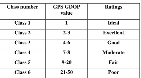
[image:1.595.311.549.193.326.2]A subset of satellites with the value of GPS GDOP less than 2 is ideal, i.e. the attained measure of location and time by these satellites are trustworthy, but a higher GPS GDOP indicates poorer satellites positioning and an inferior measurement configuration [4]. The GPS GDOP ratings are represented in Table 1 [5].
Table 1. GPS GDOP ratings Class number GPS GDOP
value
Ratings
Class 1 1 Ideal
Class 2 2-3 Excellent
Class 3 4-6 Good
Class 4 7-8 Moderate
Class 5 9-20 Fair
Class 6 21-50 Poor
To reduce the computational burden for classification and approximation of the GPS GDOP, Simon and El-Sherief have used the basic back propagation (BP) approach to train the neural network (NN) [6]. Although the BP is the most popular algorithm to train an NN, it has two important problems: 1) the BP training is very slow in many applications including the GPS GDOP classification; and 2) the BP easily falls in local minima. To overcome these problems, Jwo and Lai [1] suggested utilizing the BP with momentum to train the NN (BPNN), the optimal interpolative network, general regression NN (GRNN), and probabilistic NN (PNN). In [5] and [7] Azami et al. proposed to use some improved NN algorithms, namely, BP with adaptive learning rate and momentum, Fletcher-Reeves conjugate gradient algorithm (CGA), Polak-Ribikre CGA, Powell-Beale CGA, scaled CGA, resilient BP (RBP), Levenberg-Marquardt (LM), modified LM, one step secant (OSS) and quasi-Newton. In addition, to have uncorrelated and informative features of the GPS GDOP, principal component analysis (PCA) was used as a pre-processing step [8].
To overcome this problem, in this study we propose an approach based on neural network (NN) and evolutionary algorithms (EAs) for GPS GDOP classification. In this article we use a number of EAs including genetic algorithm (GA), particle swarm optimization (PSO), new PSO (NPSO), and imperialist competitive algorithm (ICA) to train an NN. The rest of the paper is organized as follows: Section 2 presents GPS GDOP briefly. In Section 3, EAs including genetic algorithm (GA), particle swarm optimization (PSO), new PSO (NPSO), and imperialist competitive algorithm (ICA) are explained. Section 3 describes the proposed methods. Simulation results and comparing with existing well-known methods are discussed in Section 5. Finally, Section 6 includes the conclusion of the study.
2.
THE CONCEPT OF GPS GDOP
(a)
[image:2.595.78.263.84.444.2](b)
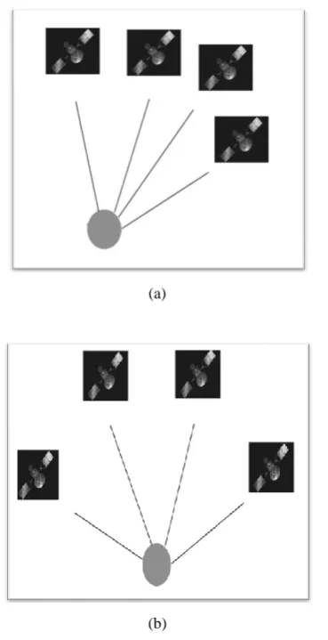
Figure 1: Satellite’s diagram and its relation with DOP: (a) Bad GDOP and (b) Good GDOP
We assume the definitions of GDOP computation, useful for the sequel of the document and help understanding our contributions. The absolute distance between a satellite and a user is defined as follows [8,9]:
,
,
trop i
iono i
Ri i
(1) where:u
t
u
Z
i
Z
u
Y
i
Y
u
X
i
X
i
(
)
2
(
)
2
(
)
2
(2)
i
iono
,
and
trop i
,
which are the errors induced by the ionospheric and the tropospheric propagation, are calculated from a model,(
X
u
,
Y
u
,
Z
u
,
t
u
)
are the four system unknowns andu
t
is the correction the receiver has to apply to its own clock. To resolve this system we need four equations which mean four pseudo-ranges from four different satellites. The pseudo-ranges can be approximated by a Taylor expansion. We obtain:
3^
^
^
^
2
2
2
(
) (
) (
)
^
X
X
Y Y
Z
Z
i
i
u
i
u
i
u
t
u
The Taylor expansion at the first order is:
^
(4)
a
x
a
y
a
z
i
i
i
xi
u
yi
u
zi
u
c t
u
where:^
^
^
;
;
;
^
^
^
^
^
^
^
2
2
2
(
)
(
)
(
)
X
X
Y
Y
Z
Z
i
u
i
u
i
u
a
a
a
xi
yi
zi
r
r
r
i
i
i
r
X
X
Y
Y
Z
Z
i
i
u
i
u
i
u
(5)
Let assume
Nsat
be the number of visible satellites. The matrixH
is as follows:
1
1
2
2
2
1
1
1
1
sat
zN
a
sat
yN
a
sat
xN
a
z
a
y
a
x
a
z
a
y
a
x
a
H
(6) Let define theG
matrix:1
)
(
H
T
H
G
(7)The GDOP is:
]
[
G
trace
GDOP
(8)
3.
EVOLUTIONARY ALGORITHMS
(EAs)
In this section we explain four mentioned EAs briefly.
3.1
Particle Swarm Optimization and New
Particle Swarm Optimization
social behavioral of animals such as birds and fish when they are together has been the inspiration source for this algorithm [10]. PSO, the same as other evolutionary algorithms, starts with a random matrix as a primary population. Unlike genetic algorithms (GA), standard PSO doesn’t have evolutionary operators like mutation and breeding. Each member of the population is named a particle. As a matter of fact, in the PSO algorithm a certain number of particles that are formed randomly make the primary values. There are two parameters for each particle including position and velocity of the particle, which are defined by a space vector and a velocity vector, respectively. These particles form a pattern in an n-dimensional space and move to the desired value. The best position of each particle in the past and the best position among all particles are stored separately. According to the experience from the preceding moves, the particles make a decision about how to decide the next move. In each iteration, all particles in the n-dimensional
problem space move to an optimum point. In each iteration, the position and velocity of each particle can be modified according to the following equations:
1 1
2 2
(
1)
( )
( )
( )
( )
( )
9
i
i
i i best i
best i
v t
wv t
C r p
t
x t
C r g
t
x t
(
1)
( )
(
1)
i i i
x t
x
t
v
t
(10) where n shows the dimension (1 ≤ n ≤ N), C1 and C2 are
positive constants, generally considered 2.0. r1 and r2 are
random numbers uniformly between 0 and 1; w is inertia weight that can be constant [11].
Equation (9) states that the velocity vector of each particle is updated (
v t
i( 1)
) and the new and previous values of thevector position (
x t
i( )
) create the new position vector (( 1)
i
x t
). As a matter of fact, the updated velocity vector influences both local and global values. The best response of the local positions is the best solution of the particle until current execution time (pbest) and the best global solution is
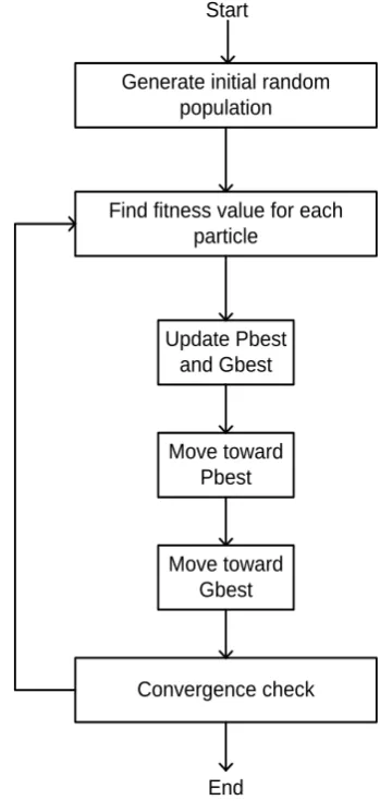
the best solution of the entire particles until current execution time (gbest). Flowchart of PSO is presented in Figure 2.
Generate initial random population
Find fitness value for each particle
Update Pbest and Gbest
Move toward Pbest
Move toward Gbest
Convergence check
[image:3.595.338.513.77.450.2]End Start
Figure 2. Flowchart of PSO
Because PSO stays in local minima of fitness function, we use NPSO. In each iteration, as it was mentioned in PSO, global best particle and local best particle are calculated. NPSO strategy uses the global best particle and local “worst” particle, the particle with the worst fitness value of the particle until current execution time [12]. It can be defined as:
1 1
2 2
(
1)
( )
( )
( )
( )
( ) (11)
i
i
i i worst i
best i
v t
wv t
C r p
t
x
t
C r g
t
x t
3.2. Genetic Algorithm
A GA has three major steps. In the first step we create an initial population of m randomly selected individuals. The first generation is created by the initial population. The second step inputs m individuals and gives as output an assessment for each of them based on an objective function known as fitness function. This evaluation explains proximity value of our demands respect to each one of these m individuals. The third step is responsible for the formulation of the subsequently generation [8,13].
operations, namely, reproduction, crossover and mutation [8,13].
In each iteration of GA, some of the individuals with highest fitness value are eliminated and replaced by new members. New members are produced by so called parents. Crossover selects probabilistically two of fittest individuals of generation N; then in a random way selects a number of their characteristics and exchanges them in a way that the selected characteristics of the first individual would be obtained by the second and vice versa. Following this procedure creates two new children that both belong to the new generation. Mutation is a physiologically-inspired disturbance to the system and is often used to avoid possible local minima. To model this for real-world optimization, initially, a random number for each bit of chromosome, then, if the random number is greater than a pre-defined “mutation threshold”, that bit is flipped. Finally, the flowchart of GA is presented in Figure 3 [8,13].
Generate initial random population
Find fitness value for each chromosome
Selection
Mating
Mutation
Convergence check
End Start
Figure 3. The flowchart of GA-based optimization cycle
3.3. Imperialist Competitive Algorithm
ICA is a new population based optimization algorithm proposed in 2007 by Atashpaz-Gargari and Lucas [14]. Nowadays ICA has numerous applications like designing controller for industrial systems, solving optimization problems in PID controller, communication systems, and training and analysis of artificial NNs [15-18].
Similar to every evolutionary algorithm, this algorithm starts with the preliminary population with random numbers that
each of them is called a "Country". A number of the members of the population that have best fitness values are chosen as imperialists. Each member of the remaining population is named a colony. Total fitness values of an empire depends on both the power of the imperialist country and the power of its colonies [13,15].
[image:4.595.84.259.269.633.2]In each step, the countries go toward their related imperialist. If the fitness value of a colony achieves more than its related fitness value of imperialist then, this colony and its related imperialist transform to imperialist and colony, respectively. In each step, the weakest colony of the weakest empire moves toward the closest empire, and the empire without any colony is eliminated. After a while, all empires fall down except for the most powerful one and all the colonies go under the control of this unique empire. Finally the flowchart of the ICA is illustrated in Figure 4 [13-16].
4.
THE GPS GDOP CLASSIFICATION
METHODS
First, in order to reduce the instruction time, all of the input and output variants become between 0 and 1 by normalizing. Since
H
T
H
is a4
4
matrix, it has four)
4
,
3
,
2
,
1
(
i
i
eigenvalues. It is clear that the four
eigenvalues for the matrix
1
)
(
H
T
H
will be
i
1
.Based on the fact that the trace of a matrix is the sum of its
eigenvalues, Equation (8) would be as below [4,5]:
1
4
1
3
1
2
1
1
GDOP
(12)
Mapping with the definition of four variants would be done as below:
)
(
4
3
2
1
)
(
1
trace
H
T
H
x
(13)
]
2
)
[(
2
4
2
3
2
2
2
1
)
(
2
trace
H
T
H
x
(14)
]
3
)
[(
3
4
3
3
3
2
3
1
)
(
3
trace
H
T
H
x
(15)
)
(
det
4
3
2
1
)
(
4
H
T
H
x
(16)
The GDOP can be considered as a mapping directly from
X
to GDOP classes. Mapping fromX
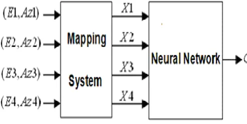
to the GDOP classes is [image:5.595.317.564.159.283.2]very non-linear and cannot be determined analytically, but it can be determined exactly by the NN. In this paper, NN is planned to do the mapping from
X
to the GPS GDOP classes. Figure 5 shows the whole classification block diagram of GPS GDOP using NN. As mentioned before in this paper we propose four EAs including ICA, GA, PSO, and NPSO.Figure 5: Classification block diagram of GPS GDOP using NN
5.
SIMULATIONS AND DISCUSSIONS
[image:5.595.73.519.497.561.2]Six classes or outputs for the proposed NNs are considered for GPS GDOP classification. When the GDOP is higher than the first threshold, NN outputs are [1 0 0] (for the large state) and when the GDOP is placed between the first and second threshold, NN outputs are [0 1 0] (for the average case) and when the GDOP is smaller than the second threshold, NN outputs are [0 0 1] (for the low state). Table 2 presents the accuracy numbers of GPS GDOP classification. Table 5 shows comparing accuracy between these three methods for GPS GDOP. The simulation results demonstrate that GPS GDOP classification using NN and ICA has better accuracy than other NN- based approaches including GA, PSO, and NPSO.
Table 2: Comparison of classification rates for proposed methods Classification
Methods
NN trained by ICA
NN trained by GA
NN trained by
NPSO NN trained by PSO BPNN [1]
Classification ratess 95.15% 94.31% 94.84% 94.17% 93.16
6.
CONCLUSIONS
GPS GDOP shows the geometrical relationship between positioning accuracy and satellite configuration. It can be calculated by using the positions of four visible satellites and the position of the receiver. The ideal GPS GDOP value is equal or less than one. Values of two to three are considered acceptable, whereas values greater than nine are considered high and should be discarded. Existing approaches for GPS GDOP approximation and classification are time-consuming and unreliable. In this paper, we propose four EAs, namely PSO, NPSO, GA and ICA, to train an NN. The simulation results demonstrate that GPS GDOP classification using NN and ICA has better accuracy than simple classification using NN and other NN-based approaches based on the EAs.
7.
REFERENCES
[1] D. J. Jwo and C. C. Lai, “Neural network-based GPS GDOP approximation and classification”, Journal of GPS Solutions, vol. 11, no. 1, pp. 51-60, 2007.
[2] M. Zhang and J. Zhang, “A fast satellite selection algorithm: beyond four satellites”, IEEE Journal of Selected Topics in Signal Processing, vol. 3, no. 5, pp. 740-747, 2009.
[3] R. Yarlagadda, I. Ali, N. Al-Dhahir and J. Hershey, “GPS GDOP metric”, IEE Proc.-Radar, Sonar Navig, vol. 147, no. 5, pp. 259-264, 2000.
[5] H. Azami, M. R. Mosavi and S. Sanei, “Classification of GPS satellites using improved back propagation training algorithms”, Wireless Personal Communications, vol. 71, no. 2, pp. 789-803, 2013.
[6] D. Simon and H. El-Sherief, “Navigation satellite selection using neural networks”, Journal of Neurocomputing, vol. 7, no. 3, pp. 247–258, 1995. [7] H. Azami and S. Sanei, “GPS GDOP classification via
improved neural network trainings and principal component analysis”, International Journal of Electronics, Taylor & Francis, http://dx.doi.org/10.1080/00207217.2013.832390, pp. 1-14, 2013.
[8] M. R. Mosavi and H. Azami, “Applying neural network ensembles for clustering of GPS satellites”, Journal of Geoinformatics, vol. 7, no. 3, pp. 7-14, 2011.
[9] M. R. Mosavi and M. Shiroie, “Efficient evolutionary algorithms for GPS satellites classification”, Arabian Journal for Science and Engineering, vol. 37, no. 7, pp. 2003-2015, 2012.
[10] L. Mussi, S. Cagnoni, and F. Daolio, “GPU-based road sign detection using particle swarm optimization”, International Conference on Intelligent Systems Design and applications, pp. 152-157, 2009.
[11] H. Azami, M. Malekzadeh and S. Sanei,“Optimization of orthogonal polyphase Coding waveform for MIMO radar based on evolutionary algorithms”, Journal of mathematics and Computer Science, vol. 6, pp. 146-153, 2013.
[12] C. Yang and D. Simon, "A new particle swarm optimization technique", International Conference on Systems Engineering, pp. 164-169, 2005.
[13] H. Azami, S. Sanei, K. Mohammadi and H. Hassanpour, “A hybrid evolutionary approach to segmentation of non-stationary signals”, Digital Signal Processing, vol. 23, no. 4, pp. 1103-1114, 2013.
[14] E. Atashpaz-Gargari and C. Lucas, “Imperialist competitive algorithm: an algorithm for optimization inspired by imperialistic competition”, IEEE Congress on Evolutionary Computation, pp. 4661-4666, 2007. [15] M. Abdechiri, K. Faez and H. Bahrami, “Neural network
learning based on chaotic imperialist competitive algorithm”, 2nd International Intelligent Systems and Applications (ISA), pp. 1-5, 2010.
[16] E. Atashpaz-Gargari, F. Hashemzadeh, R. Rajabioun and C. Lucas, “Colonial competitive algorithm: a novel approach for PID controller design in MIMO distillation column process”, International Journal of Intelligent Computing and Cybernetics, vol. 1, no. 3, pp. 337-355, 2008.
[17] R. Rajabioun, E. Atashpaz-Gargari and C. Lucas, "Colonial competitive algorithm as a tool for Nash equilibrium point achievement", Lecture Notes in Computer Science, pp. 680-695, 2008.