Extension of PROMETHEE Method for Solving Multi Objective Optimization Problems

Extension of PROMETHEE method for solving multi

objective optimization problems

Mansoureh Maadi

Damghan university Damghan, Iran

Marzieh Soltanolkottabi

Isfahan University of Technology Isfahan, Iran

ABSTRACT

The most methods used for solving multi objective optimization problems (MOPs) are based on the Pareto-optimal frontier, but this approach will become questionable when the number of objectives grows. This paper presents an approach for solving MOPs using PROMETHEE method (Preference Ranking Organization methods for Enrichment Evaluation). In this paper the optimal solution of MOPs is built base on minimizing the preference of positive ideal solution and maximizing the preference over negative ideal solution. Thus, a k-dimensional objective space is reduced to a two-dimensional space. The concept of membership function of fuzzy set theory is used to represent the satisfaction level for both criteria and a max-min operator is used for solving the transformed problem. Finally a numerical example is illustrated.

General Terms

Computational Mathematics, Decision making.

Keywords

Multiobjective Optimization Problem (MOP), PROMETHEE method, Preference function, Fuzzy set theory.

1.

INTRODUCTION

Decision making is the process of selecting the best possible alternatives among all alternatives and multi criteria decision making is often related to ranking of many alternatives from the best to the worst based on multiple conflicting criteria. Multi objective optimization is the process of optimizing two or more objects that are often conflicted to each other. The choice of the final solution of MOP can be stated as a typical multi criteria decision problem determining which is the best among all possible efficient solutions, according to the decision maker (DM) preferences, taking into account several criteria [1].

In the literature there are several methods that combine decision methods with optimization algorithms in order to determining the final solution of MOPs [1, 2, 3]. Generally these methods can be classified into three groups: the a priori, a progressive and a posteriori decision making. In a priori decision making, DM is consulted before the optimization process only one time and the optimization process continue until it reach to final optimum solution. In the progressive decision making the DM’s preference is repeatedly used in the course of the optimization process in order to guide the search algorithm. Finally, a posterior decision making method starts with the execution of a multi objective optimization algorithm in order to find some acceptable solution and after that DM is

consulted to compare the available alternatives and choose a unique final solution.

PROMETHEE is one of the popular decision making methods which has been successfully applied in the selection of the final solution of convex MOPs [4]. This method was first developed by Brans in 1982 [5]. PROMETHEE method generates a ranking of available points according to the DM’s preference and finally presents a unique final solution. This method is based on a pair-wise comparison of alternatives along each criterion. Alternatives are compared according to different criteria after they will be ranked. There are many papers that applied PROMETHEE methods in methodologies and applications and the number of papers increases year by year [5].

In the literature there are some articles that applied PROMETHEE methods to find the most satisfactory optimal solution of a multiobjective program [6, 7]. Application of PROMETHEE method in these articles related to posteriori methods in finding solution of MOPs. In [7] a posteriori decision multiobjective optimization problems with smarts, PROMETHEE II and a fuzzy algorithm is investigated and compared. In [6], R.O.Parreiras and J.A.Vasconcelos presented a multiplicative version of PROMETHEE II and applied that in multi objective problems. In these two articles after finding Pareto-optimal frontier, the PROMETHEE method applied to finding the most satisfactory optimal solution of MOPs. Also Martel and Aouni presented a method to find the optimal solution of a goal programming model [8]. After that Diaby and Martel developed a new goal programming approach combined with the PROMETHEE to model the decision-maker preferences [9].

In the literature some methods are applied with PROMETHEE method such as AHP, ELECTRE, and so on [10, 11, 12, 13]. In many papers PROMETHEE method is compared with other MCDM methods and in some articles PROMETHEE methods and fuzzy set theory are applied together [14, 15, 16]. For example [14] present an extension of the PROMETHEE method for decision making in fuzzy environment. In these articles input data in PROMETHEE method are fuzzy numbers.

2.

PROMETHEE METHOD

PROMETHEE is a multi-criteria decision making method developed by Brans in 1982. A few years later, several versions of the PROMETHEE method developed. These methods are:

 PROMETHEE II for complete ranking of alternatives,

 PROMETHEE III for ranking based on intervals,

 PROMETHEE IV for complete or partial ranking of the alternatives,

 PROMETHEE V for problems with segmentation constraints,

 PROMETHEE VI for the human brain representation,

 PROMETHEE GDSS for group decision- making,

 PROMETHEE & GAIA for graphical representation,

 PROMETHEE TRI for dealing with sorting problems and

 PROMETHEE CLUSTER for nominal

classification [5].

PROMETHEE method is a ranking method that is simple in application compared to other MCDM methods. This method is well adapted to problems which some alternatives are to be ranked considering several criteria.

The implementation of PROMETHEE needs three types of information:

1- Evaluation table: the table of alternatives and criterions such as follow:

Table 1 Evaluation table

a g1(. ) g2(. ) … gk(. )

a1 g1(a1) g2(a1) … gk(a1)

a2 g1(a2) g2(a2) … gk(a2)

⋮ ⋮ ⋮ ⋮ ⋮

an g1(an) g2(an) … gk(an)

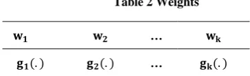
In this table a1, a2, … , anare alternatives and g1 . , g2 . , … , gk(. ) are criterion and the goal is finding the most satisfactory alternative according to criterions. 2- Weights (information on the relative importance of the criteria): this method assumes that DM is able to weight the criteria and doesn’t have specific guide for determining weights. In the literature several methods for determining weights are declared [17, 18].

Table 2 Weights

3- The preference function: the preference function (pi) is defined for every criterion and is used to compare the contribution of the alternatives in terms of each separate criterion. It reflects the preference level of alternative “a” over “b” in the interval [0 1].

Table 3 Preference function

𝐩𝟏(. , . ) 𝐩𝟐(. , . ) … 𝐩𝐤(. , . )

𝐠𝟏(. ) 𝐠𝟐(. ) … 𝐠𝐤(. )

The steps of PROMETHEE method can be stated as follows: 1: determination of deviations based on pair-wise

comparisons of two alternatives:

dj a, b = gj a − gj b

Where dj(a, b) is the difference of the value of “a” and “b” in each criterion.

2: application of preference function:

pj a, b = Fj[dj a, b ]

Where pj a, b denotes the preference of alternative “a” with regard to alternative “b” in each criterion, as a function of dj a, b . In order to facilitate the selection of a specific preference function, six basic types have been proposed [19]. 3: calculation of global preference index:

∀ a, b ϵA π a, b = kj=1pj a, b wj

Where π a, b is defined as the weighted sum of pj a, b for each criterion.

4: calculation of outranking flows as follow:

Φ+ _{a =} 1

n−1 xϵAπ(a, x)

Φ− _{a =} 1

n−1 xϵAπ(x, a)

Where Φ+ a and Φ− a are positive outranking flow and negative outranking flow for each alternative.

This step is the final step of PROMETHEE I. In this method alternative “a” is superior to alternative “b” if the positive flow of “a” is greater than the positive flow of “b” and the negative flow of “a” is smaller than the negative flow of “b”.

3. PROPOSED METHOD

Consider a multi objective optimization problem (MOP) as follow:

max (or min) F X = f1 X , f2 X , … , fn X

subject to S = gi X

≤ ≥

= 0 ; i = 1, 2, … , m X ∈ EN

(1)

Where X = (x1, x2, . . . , xN) and the objective functions and the system of constraints are convex real valued functions on Rn.

𝐰𝟏 𝐰𝟐 … 𝐰𝐤

Assume that for each k = 1, 2, … , n, we have

fk+= max (or min) fk(X) | X ∈ S (2a)

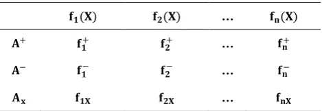
fk−= min (or max) fk(X) | X ∈ S (2b) Regarding above definition, two alternatives A+ and A− are identified and optimal solution can be built in comparison with them, as in PROMETHEE method. So the decision area for PROMETHEE method is as follow:

Table 4 Decision area for PROMETHEE method

In table 4, Ax is the optimal solution which should be built and now it is considered in parametric form.

As in PROMETHEE method d should be calculated according to mentioned definition, in proposed method d which denotes the difference between the evaluations of two alternatives on each objective is defined as follows:

dk A+, AX = fk+− fkX (3a)

dk AX , A− = fkX− fk− (3b) The preference functions will be used to demonstrate the preference of one alternative to another.

Pk A+, AX = Fk(dk A+, AX ) (4a)

Pk AX , A− = Fk(dk AX , A− ) (4b)

Fig 1: Gaussian preference functions

Then the overall preference of one alternative over another will be calculated. wk will be determined by DMs.

π A+_{, A}

X = nk=1wkPk A+, AX (5a)

π AX , A− = nk=1wkPk AX , A− (5b) As described in part 2, there are two different outranking

flows, positive and negative. For each x ∈ S and k =

1, 2, … , n, the value of f_k+ is preferred to the value of fkx. So, the positive outranking flow in this problem will calculate from the next equation.

Φ+ AX = π AX , A− (6a) the same as positive outranking flow, for each x ∈ S and k =

1, 2, … , n, the value of fkx is preferred to the value of fk−, therefore the following equation will represent the value of negative outranking flow.

Φ− AX = π A+, AX (6b) Following the PROMETHEE I method, the larger value for

Φ+ Ax and the smaller value forΦ− Ax are preferred, so, the MOP can be replaced by the following formulation:

min Φ− AX

max Φ+ AX

subject to X ∈ S (7a) Or

min π A+_{, A} X

max π AX , A−

subject to X ∈ S (7b) or

min wk n

k=1

Pk A+, AX

max wk n

k=1

Pk AX , A−

subject to X ∈ S (7c) Thus, by the previous formulation, a k-dimensional objective space is reduced to a two-dimensional space.

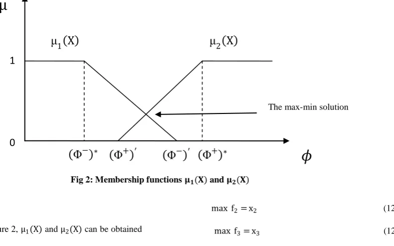
These two objectives are usually conflicting to each other. In order to solve this problem membership functions can be used which represent these two objectives individual optima. Assume that the membership functions μ1(X) and μ2(X) of two objective functions are linear between (Φ)∗_and

Φ ,′_{which are:}

(Φ−)∗_{= {min Φ}− _A

X | X ∈ S} and the soloution is X− (8a)

(Φ+)∗_{= {max Φ}+ _A

X | X ∈ S} and the soloution is X+ (8b)

(Φ−)′_=Φ− _A

X+ (8c)

(Φ+)′_=Φ+ _A

X− (8d)

𝐟𝟏(𝐗) 𝐟𝟐(𝐗) … 𝐟𝐧(𝐗)

𝐀+ _𝐟

𝟏+ 𝐟𝟐+ … 𝐟𝐧+

𝐀− _𝐟

𝟏− 𝐟𝟐− … 𝐟𝐧−

𝐀𝐱 𝐟𝟏𝐗 𝐟𝟐𝐗 … 𝐟𝐧𝐗

d

1

Fig 2: Membership functions 𝛍𝟏(𝐗) and 𝛍𝟐(𝐗)

Then, as shown in Figure 2, μ1(X) and μ2(X) can be obtained as follow:

μ₁ X =

1 if Φ− _A

X < (Φ−)∗

1 −Φ− AX − Φ−∗

Φ−′₋ Φ−∗ if (Φ

−₎∗_{≤ Φ}− _A

X ≤ (Φ−)′

0 if (Φ−)′_<Φ− _A

X

(9a)

μ₂ X =

0 if Φ+ _A

X < (Φ+)′

1 − Φ+∗−Φ− AX

Φ+∗− Φ+′ if (Φ

+₎′_{≤ Φ}+ _A

X ≤ (Φ+)∗

1 if (Φ+₎∗_<Φ+ _A

X

(9b)

Now, by applying the max–min decision model which is proposed by Bellman and Zadeh and extended by Zimmermann [20], the transformed problem can be resolved. Assume that the satisfying decision may be obtained from the following problem:

μ X∗ _{= max}

X∈S{min(μ1 X , μ2 X )} (10) If δ = min⁡(μ1 X , μ2 X ), then the model will be

transformed to the following model:

max δ

subject to μ1 X ≥ δ and μ2 X ≥ δ (11)

XϵS δϵ[0,1]

It is well known that the optimal solution of this problem is the answer of MOP.

4. AN EXAMPLE

Step0. Consider the following multi objective optimization problem

max f1= x1 (12a)

max f2= x2 (12b)

max f3= x3 (12c)

subject to 5x1+ 3x2+ 2x3≤ 240

3x3+ x1≤ 320 (12d)

2x1+ 3x2+ 4x3 ≤ 180

X ≥ 0

Step1. Calculation of f_k+and f_k−as shown in table 5 and 6.

Table 5 Calculation of 𝐟𝐤+

𝐟𝟏 𝐟𝟐 𝐟𝟑 𝐱𝟏 𝐱𝟐 𝐱𝟑

𝐦𝐚𝐱 𝐟𝟏 48* 0 0 48 0 0

𝐦𝐚𝐱 𝐟𝟐 0 60* 0 0 60 0

𝐦𝐚𝐱 𝐟𝟑 0 0 45* 0 0 45

f+_{= 48, 60, 45}

Table 6 Calculation of 𝐟𝐤−

𝐟𝟏 𝐟𝟐 𝐟𝟑 𝐱𝟏 𝐱𝟐 𝐱𝟑

𝐦𝐢𝐧 𝐟𝟏 0* 0 0 0 0 0

𝐦𝐢𝐧 𝐟𝟐 0 0* 0 0 0 0

𝐦𝐢𝐧 𝐟𝟑 0 0 0* 0 0 0

f−_{= 0, 0, 0}

Φ

Φ

_Φ

_Φ

μ

μ

X

μ

X

The max-min solution

1

𝜙

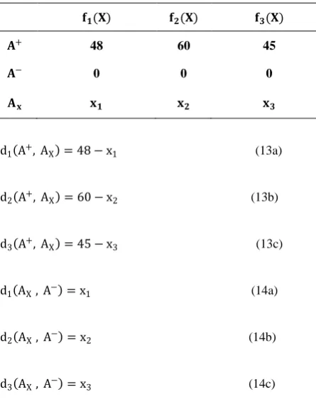
Step2. Calculation of d by using table 7. In this table three alternatives A+, A− and Ax are obtained.

Table 7 Decision area

𝐟𝟏(𝐗) 𝐟𝟐(𝐗) 𝐟𝟑(𝐗)

𝐀+ _{48 60 45}

𝐀− _{0 0 0}

𝐀𝐱 𝐱𝟏 𝐱𝟐 𝐱𝟑

d1 A+, AX = 48 − x1 (13a)

d2 A+, AX = 60 − x2 (13b)

d3 A+, AX = 45 − x3 (13c)

d1 AX , A− = x1 (14a)

d2 AX , A− = x2 (14b)

d3 AX , A− = x3 (14c)

Step3. Next, preferences will be calculated for each d. The preference functions for f1(X), f2 X and f3(X) are assumed as follows:

Preferences function for f1(X):

Fig3: Preference function for 𝐟𝟏(𝐗)

P1 d =

0 d ≤ 2

d−2

10−2 2 < 𝑑 ≤ 10

1 d > 10

(15)

Preference function for f2(X):

Fig 4: Preference function for 𝐟𝟐(𝐗)

P2 d =

0 d ≤ 5

d−5

15−5 5 < 𝑑 ≤ 15

1 d > 15

(16)

Preference function for f3(X):

Fig 5: Preference function for 𝐟𝟑(𝐗)

P3 d =

0 d ≤ 2

d−2

10−2 2 < 𝑑 ≤ 10

1 d > 10

(17)

In order to insert these formulas to the optimization problem, it is needed to transform them to the following formulas:

Transformed forms of preference function for f1(X):

1

16( d1− 2 − d1− 10 + 8)

subject to 0 ≤ d1 (18)

Transformed form of preference function for f2(X)

1

20( d2− 5 − d2− 15 + 10)

subject to 0 ≤ d2 (19)

2

10

𝑃

5

15

𝑃

2

10

Transformed form of preference function for f3(X)

1

16( d3− 2 − d3− 10 + 8)

subject to 0 ≤ d3 (20)

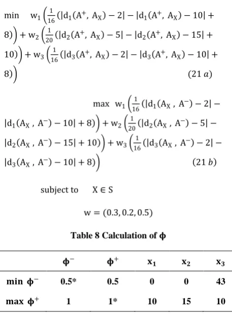
Step4. In this step, preference functions should be placed in equation (7c) to make the transformed form of MOP. wiwill be determine by DMs. Then the value of (Φ−)∗ , (Φ−)′,

(Φ+)∗ _{and (Φ}−₎∗ _{are obtained by solving this problem.}

These values are illustrated in table 8.

min w1 ₁₆1 d1 A+, AX − 2 − d1 A+, AX − 10 +

8 + w2 ₂₀1 d2 A+, AX − 5 − d2 A+, AX − 15 +

10 + w3 ₁₆1 d3 A+, AX − 2 − d3 A+, AX − 10 +

8 (21 𝑎)

max w1 ₁₆1 d1 AX , A− − 2 −

d1 AX , A− − 10 + 8 + w2 ₂₀1 d2 AX , A− − 5 −

d2 AX , A− − 15 + 10 + w3 ₁₆1 d3 AX , A− − 2 −

d3 AX , A− − 10 + 8 21 𝑏

subject to X ∈ S

w = (0.3, 0.2, 0.5)

Table 8 Calculation of 𝛟

𝛟− _𝛟+ _𝐱

𝟏 𝐱𝟐 𝐱𝟑

𝐦𝐢𝐧 𝛟− _{0.5* 0.5 0 0 43}

𝐦𝐚𝐱 𝛟+

1 1* 10 15 10

Step5. In order to solve the problem by means of max-min operator, μ₁ X and μ₂ X are calculated as explained. Finally the solution of MOP is found by computing (11) which is the fuzzy form of the previous problem.

μ₁ X =

1 if Φ− AX < 0.5

1 −Φ− AX −0.5

1−0.5 if 0.5 ≤ Φ − _A

X ≤ 1

0 if 1 <Φ− _A

X

(22a)

μ₂ X =

0 if Φ+ _A

X < 0.5

1 − Φ+∗−Φ− AX

Φ+∗− Φ+′ if 0.5 ≤ Φ

+ _A

X ≤ 1

1 if 1 <Φ+ _A

X

(22b)

max δ

subject to 1 −Φ

− _A X − 0.5

1 − 0.5 ≥ δ

1 −1−Φ

− _A X

1 − 0.5 ≥ δ

XϵS δϵ[0,1] (23) The maximum satisfactory level is achieved for the

solution X = (44, 0, 10).

5. CONCLUSION

In this paper, a PROMETHEE approach has been extended to solve multi objective optimization problems. This approach provides a way to find the satisfactory solution of MOP. It transfers k-objectives optimization problem, into two objectives optimization problem by minimizing the preference of positive ideal solution and maximizing the preference over negative ideal solution, which will be practical when the number of objectives increases. Also, by using Piecewise linear segmentation, the preference functions can be entered into the model thus, multi objective nonlinear optimization problems can be solved. Other fuzzy operators can be used for solving the transformed bi-objective optimization problem.

6. REFERENCES

[1] R.O. Parreiras, J.A. Vasconcelos, 2005, Decision making in multiobjective optimization problem, Nedjah Nadia, Mourelle Luiza de Macedo (Eds.), ISE Book Series on Real word Multi-objective system Engineering, Nova science, New York, USA, ,1-20.

[2] J. Horn, 1997, Multi criterion decision making, Thomas Bӓck, David Fogel, Zbigniew Michalewicz (Eds.), Handbook of Evolutionary Computation, IOP Publishing Ltd. And Oxford University Press, New York, USA, , pp. F1.9:1-F1.9:15.

[3] C.A.C. Coello, 2000. handling preferences in evolutionary multi objective optimization: A survey, In Proceedings of the 2000 congress on Evolutionary computation, IEEE servic.

[4] J.p. Brans, Ph. Vincke, B. Mareschal, "How to select and how to rank projects: The PROMETHEE method", European journal of operational research 24(1986) 228-238.

[5] M. behzadian, R.B. kazemzadeh, A. Albadvi, M. Aghdasi, "PROMETHEE: a comprehensive literature review on methodologies applications", European journal of operational research 200 (2010) 198-215.

[6] R.O. Parreiras, J.A. Vasconcelos, "A multiplicative version of PROMETHEE Π applied to multi objective optimization problems", European journal of operational research 183 (2007) 729-740.

[7] R.O. Parreiras, J.H.R.D. Maciel, J.A. Vasconcelos, "The a posteriori decision in multiobjectve optimization problems with smarts, PROMETHEE II , and a fuzzy algorithm", IEEE Transactions on magnetic, vol. 42,No.4 (2006).

[9] M.Diaby, J.M.Martel, "Preference structure modeling for multi-objective decision making: A goal-programming approach". Journal of Multi-Criteria Decision Analysis 6 (1997) 150–154.

[10] W.jianjun and Y.Delli, "an AHP/PROMETHEE based method of selecting supplier", CNKI journal, cnki: ISSN: 1003-1952.0.2006-07-011 (2006).

[11] M. Dagdeviren, "Decision making in equipment selection: An integrated approach with AHP and PROMETHEE", J Intell Manuf (2008) 19:397–406.

[12] J.J. Wang, C.M. Wei, D.L. Yang, "Decision method for vendor selection based on AHP\PROMETHEE\ GAIA". Dalian ligong Dauxe xuebao, Journal of Dalian university of technology 46(6) (2006) 926-931.

[13] C. Macharis, j. Springael, K.D. Brucker, A. Verbeke, "PROMETHEE and AHP: The design of operational synergies in multi criteria analysis", European journal of operational research 153 (2004) 307-317.

[14] M. Goumas, V. Lygerou," An extension of the PROMETHEE method for decision making in fuzzy environment: Ranking of alternative energy exploitation projects". European journal of operational research 123 (2000) 606-613.

[15] J. Geldermannn, T. Spengler, O. Rentz, "Fuzzy outranking for environmental assessment. Case study: Iron and steel making industry". Fuzzy sets and systems 115 (2000) 45-65.

[16] J.f. Le Teno, B. Mareschal, "An interval version of PROMETHEE for the comparison of building products’ design with ill-defined data on environmental quality", European journal of operational research ,109 (1998) 522-529.

[17] Ch. Kao, "Weight determination for consistently ranking alternatives in multiple criteria decision analysis", Applied Mathematical Modeling 34 (2010) 1779–1787.

[18] Y.M. Wang, Y. Luo, "Integration of correlations with standard deviations for determining attribute weights in multiple attribute decision making", Mathematical and Computer Modeling 51 (2010) 1-12.

[19] J. Figueira, S. Greco, M. Ehrgott," Multiple Criteria Decision Analysis": State of the Art Surveys. Springer Verlag, Boston, Dordrecht, London, 2005.