The Odd Generalized Exponential Gompertz Distribution

(1)

http://dx.doi.org/10.4236/am.2015.614206

The Odd Generalized Exponential

Gompertz Distribution

M. A. El-Damcese

1

_{, Abdelfattah Mustafa}

2

_{, B. S. El-Desouky}

2

_{, M. E. Mustafa}

2

1_{Department of Mathematics, Faculty of Science, Tanta University, Egypt} 2_{Department of Mathematics, Faculty of Science, Mansoura University, Egypt}

Received 6 November 2015; accepted 28 December 2015; published 31 December 2015

This work is licensed under the Creative Commons Attribution International License (CC BY).

http://creativecommons.org/licenses/by/4.0/

Abstract

In this paper we propose a new lifetime model, called the odd generalized exponential gompertz distribution. We obtained some of its mathematical properties. Some structural properties of the new distribution are studied. The method of maximum likelihood is used for estimating the model parameters and the observed Fisher’s information matrix is derived. We illustrate the usefulness of the proposed model by applications to real data.

Keywords

Gompertz Distribution, Hazard Function, Moments, Maximum Likelihood Estimation, Odds Function, T-X Family of Distributions

1. Introduction

(2)

Recently, a generalization of the Gompertz distribution based on the idea given in [3] was proposed by [4] this new distribution is known as generalized Gompertz (GG) distribution which includes the exponential (E), generalized exponential (GE) and Gompertz (G) distributions. A new generalization of th Gompertz (G) distri-bution which results of the application of the Gompertz distridistri-bution to the Beta generator proposed by [5], called the Beta-Gompertz (BG) distribution which introduced by [6]. On the other hand the two-parameter exponen-tiated exponential or generalized exponential distribution (GE) introduced by [3]. This distribution is a particular member of the exponentiated Weibull (EW) distribution introduced by [7]. The GE distribution is a right skewed unimodal distribution, the density function and hazard function of the exponentiated exponential distribution are quite similar to the density function and hazard function of the Gamma distribution. Its applications have been wide-spread as model to power system equipment, rainfall data, software reliability and analysis of animal be-havior.

Recently [8] proposed a new class of univariate distributions called the odd generalized exponential (OGE) family and studied each of the OGE-Weibull (OGE-W) distribution, the OGE-Fréchet (OGE-Fr) distribution and the OGE-Normal (OGE-N) distribution. This method is flexible because the hazard rate shapes could be in-creasing, dein-creasing, bathtub and upside down bathtub.

In this article we present a new distribution from the exponentiated exponential distribution and gompertz distribution called the Odd Generalized Exponential-Gompertz (OGE-G) distribution using new family of un-ivariate distributions proposed by [8]. A random variable X is said to have generalized exponential (GE) distri-bution with parameters α β, if the cumulative distribution function (CDF) is given by

( )

(

1 e x

)

, 0, 0, 0.

F x = − −α β x> α > β > (1) The Odd Generalized Exponential family by [8] is defined as follows. Let G x

( )

; is the CDF of any distri-bution depends on parameter  and thus the survival function is G x

( )

, = −1 G x

( )

; , then the CDF of OGE- family is defined by replacing x in CDF of GE in Equation (1) by

( )

;,

G x G x



 to get

(

)

( )( );,

; , , 1 e , 0, 0, 0, 0.

G x G x

F x x

β α

α β = − −  > α> > β >

 

 

 

  (2)

This paper is outlined as follows. In Section 2, we define the cumulative distribution function, density func-tion, reliability function and hazard function of the Odd Generalized exponential-Gompertz (OGE-G) distribu-tion. In Section 3, we introduce the statistical properties include, the quantile function, the mode, the median and the moments. Section 4 discusses the distribution of the order statistics for (OGE-G) distribution. Moreover, maximum likelihood estimation of the parameters is determined in Section 5. Finally, an application of OGE-G using a real data set is presented in Section 6.

2. The OGE-G Distribution

2.1. OGE-G Specifications

In this section we define new four parameters distribution called Odd Generalized Exponential-Gompertz dis-tribution with parameters α λ β, , ,c written as OGE-G(Θ), where the vector Θ is defined by Θ =

(

α λ β, , ,c

)

.

A random variable X is said to have OGE-G with parameters α λ, , ,cβ if its cumulative distribution function given as follows

(

)

( )

e 1

; 1 e , 0, , , , 0,

cx c

F x x c

λ β

α

α λ β −

 

 

− _ −_

 

 

 

 

Θ =_ − _ > >

 

 

(3)

where α λ, ,c are scale parameters and β is shape parameter.

2.2. PDF and Hazard Rate

(3)

(

)

( )

e 1

( )

e 1

1

e 1 e 1

e 1

; e e e 1 e ,

cx cx

c c

cx

cx c

f x

λ λ β

α α

λ

αβλ

− − −

   

   

− _ −_ − _ −_

− __ __ __ __

 

 

Θ = _ − _

 

 

(4)

where x>0, , , ,α λ cβ >0.

A random variable X ~ OGE-G

( )

Θ has survival function in the form

( )

e 1

1 1 e .

cx c

S x

λ β

α − 

− _ −_

 

 

 

 

= − −_ _

 

 

(5)

The hazard rate function of OGE-G

( )

Θ is given by

( )

_{( )}

( )

e 1 e 1

e 1

1

e 1 e 1

e 1

e e e 1 e

.

1 1 e

cx cx

c c

cx

cx c

f x h x

S x

λ λ

λ

β

α α

λ

β α

αβλ

− −

−

   

   

− _ −_ − _ −_

− __ __ __ __

 

 

− _ −_

 

 

 

 

 ₋ 

 

 

 

= =

 

 

− − 

 

 

(6)

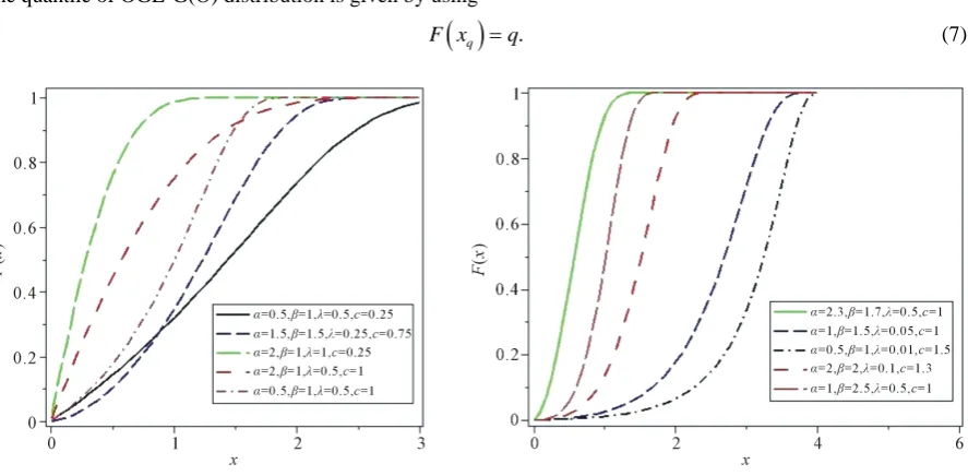
[image:3.595.81.542.80.357.2] [image:3.595.95.539.488.706.2]

The cumulative distribution, probability density and hazard rate function of the OGE-G(Θ) are displayed is

Figure 1,Figure 2 andFigure 3.

It is clear that the hazard function of the OGE-G distribution can be either decreasing, increasing, or of bath-tub shape, which makes the distribution more flexible to fit different lifetime data set.

3. The Statistical Properties

In this section, we study some statistical properties of OGE-G, especially quantile, median, mode and moments.

3.1. Quantile and Median of OGE-G

The quantile of OGE-G(Θ) distribution is given by using

( )

_q .

F x =q (7)

(4)

[image:4.595.67.544.80.273.2] [image:4.595.189.439.297.478.2]

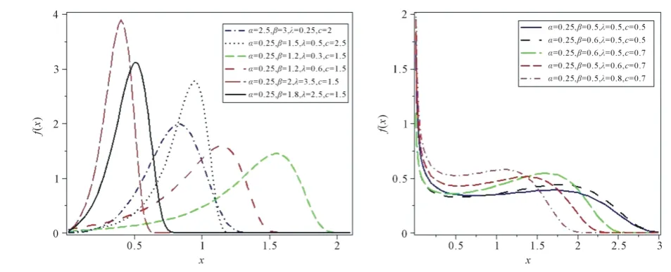
Figure 2. The pdf’s of various OGE-G distributions for some values of the parameters.

Figure 3. The hazard of various OGE-G distributions for some values of the parameters.

Substituting from (3) into (7), x_q can be obtained as

1

1 1

ln 1 ln 1 ln 1 , 0 1.

q

c

x q q

c

β

λ α

   

 _ _

=  + − _ − _  < <

 

   

 

(8)

The median of a random variable X that has probability density function f x

( )

is a number x_m such that

( )

d

[

]

0.5

m

x

m

f x x P X x

−∞ = ≤ =

∫

Therefore the median of OGE-G (α λ, , ,cβ) distribution can be obtained by setting q = 0.5 (50% quantile) in (8). 1

1 1 1

ln 1 ln 1 ln 1 .

2

c Med

c

β

λ α

   

 _ _   __

=  + _ − _ − _{ } __

 __ _ ___

 

(9)

3.2. The Mode of OGE-G

(5)

and equal it to zero thus the mode of the OGE-G(Θ) distribution can be obtained as a nonnegative solution of the following nonlinear equation

( )

e

( )

e 1 1

₍

₎

( )

e

( )

e 1 1

e 1 e 1

e e e 1 e 1 e e e 0.

cx cx

c c

cx cx

cx cx c cx c

c

λ λ

α α

λ λ

λ αλ αλ β

− −         − _ −_ − _ −_ − __ __ − __ __      _{ } _ + −  − + − =           (10)

FromFigure 2, the pdf for OGE-G distribution has only one peak. It is a unimodal distribution, so the above equation has only one solution. It is not possible to get an explicit solution of (10) in the general case. Numerical methods should be used such as bisection or fixed-point method to solve it.

3.3. The Moments

Moments are necessary and important in any statistical analysis, especially in applications. It can be used to study the most important features and characteristics of a distribution (e.g., tendency, dispersion, skewness and kurtosis). In this subsection, we will derive the rth moments of the OGE-G(Θ) distribution as infinite series ex-pansion.

Theorem 1. If X ~ OGE-G

( )

Θ , where Θ =

(

α λ, , ,cβ

)

, then the rth moment of X is given by

( )

(

) (

)

(

)

1 1 1 1 1

0 0 0 0 0

1 1 1 !

1 .

! ! 1

j j

j

i j k m

r _r r

i j k m

j i j k r

i m k c j m

β _β _{α βλ}

µ − ∞ ∞ + + + + +

+ + + = = = = = − + − +     ′ = − _ _{  } − +    

∑∑∑∑ ∑

 _      

Proof. The rth moment of the random variable X with pdf f x

( )

is defined by

( )

0 d .

r r x f x x

µ

′ =

_∫

∞ (11) Substituting from (4) into (11), we get

( )

e 1

( )

e 1

1

e 1 e 1

e 1

0 e e e 1 e d .

cx cx

c c

cx

r cx c

r x x

λ λ β

α α λ µ αβλ − − −         − _ −_ − _ −_ − ∞ __ __ __ __     ′ = _ − _    

∫

(12)

Since

( )

e 1

0 1 e 1

cx c λ

α − 

− _ −_

 

 

< − < for x>0, we have

( )

e 1 e 1

1

e 1 ₁ e 1

0

1

1 e 1 e .

cx cx

c i c

i i i

λ β λ

α − _β _β α −

−         − _ −_ ₋ − _ −_         =      −   ₋  ₌ ₋            

∑

(13)

Substituting from (13) into (12), we obtain

( )

e 1

1 e 1

1 _e ₁

0 0

1

1 e e e d .

cx c cx i

i r cx c r i x x i λ α λ β _β µ αβλ −     − + − − ∞ − __ __ = −   ′ = _{− } _  

∑

∫

Using the series expansion of

( )

e 1

1 e 1

e

cx c

i

λ

α  − 

− + _ −_

 

 _{, we get}

( )

(

)

( )

1 _e ₁ _e ₁

0

0 0

1 1

1 e e e 1 d .

!

cx cx j

j j

i j r cx c c

r i j i x x i j λ λ

β _β _α

µ − ∞αβλ + ∞ − −

= =   − +   ′ = −   _ − _    

∑∑

∫

Using binomial expansion of e

( )

e 1 1

cx j c λ ₋   −    

(6)

( )

1

(

)

( )

1 _{1 e} ₁

0 0 0 0

1 1

1 e e d .

!

cx

j j

j _{j k}

i j k r cx c r

i j k

j i

x x

i k j

λ

β _β _{α βλ}

µ − ∞ + + + ∞ − + −

= = = − +    ′ = − _ _{ }   

∑∑∑

∫

Using series expansion of e ( 1 e)

( )

1

cx

j k c

λ _{− +} ₋

, we get

( )

(

) (

)

(

)

( )

(

) (

)

( )

1 1 1

0 0 0 0 0

1 1 1

1 0

0 0 0 0 0

1 1 1

1 e e 1 d ,

! !

1 1 1

1 e d .

! !

j j

j

i j k r cx cx

r

i j k

j j

j

i j k m r c m x

i j k m

j i j k

x x

i k c j

j i j k

x x

i m k c j

β

β α βλ

µ

β α βλ

+ + − ∞ ∞ _{+ +} _∞ = = = = + + − ∞ ∞ _{+ + +} _∞ − + = = = = = − + − +    ′ = − _ _{ } −    − + − +     = − _ _{  }    

∑∑∑∑

∫

∑∑∑∑ ∑

∫

             

By using the definition of gamma function in the form

( )

1

0e d , , 0.

z tx z

z x ∞ t − t z x

Γ =

_∫

>

Thus we obtain the moment of OGE-G(Θ) as follows

( )

(

) (

)

(

)

1 1 1 1 1

0 0 0 0 0

1 1 1 !

1 .

! ! 1

j j

j

i j k m

r _r r

i j k m

j i j k r

i m k c j m

β _β _{α βλ}

µ − ∞ ∞ + + + + +

+ + + = = = = = − + − +     ′ = − _ _{  } − +    

∑∑∑∑ ∑

 _      

This completes the proof.

4. The Order Statistic

Let X X₁, ₂,,Xn be a simple random sample of size n from OGE-G(Θ) distribution with cumulative

distribu-tion funcdistribu-tion F x

(

;Θ

)

and probability density function f x

(

;Θ

)

given by (3) and (4) respectively. Let

1:n 2:n n n:

X ≤X ≤≤X denote the order statistics obtained from this sample. The probability density function of

:

r n

X is given by

(

)

₍

_{) (}

)

1

(

)

(

)

:

1

, , 1 , ; ,

, 1

r n r

r n

f x F x F x f x

B r n r

− −

Θ = _ Θ _ _ − Θ _ Θ

− + (14)

where f x

(

;Θ

)

and F x

(

,Θ

)

are the pdf and cdf of OGE-G(Θ) distribution given by (3) and (4) respectively and B

( )

.,. is the beta function. Since 0<F x

(

,Θ <

)

1 for x>0, we can use the binomial expansion of

(

)

1−F x,Θ n r−

 

  given as follows

(

)

( )

(

)

0

1 , 1 , .

n r

n r i i

i

n r

F x F x

i − − = −  

− Θ = − Θ

  _ _  

 

∑

_ _   (15)

Substituting from (15) into (14), we have

(

)

₍

_{) (}

)

( )

(

)

1

:

0

1

, ; 1 , .

, 1

n r _{i r} i

r n

i

n r

f x f x F x

i B r n r

− _{+ −}

=

−

 

Θ = Θ _ _ − _ Θ _

− +

∑

_ _ (16)

Substituting from (3) and (4) into (16), we obtain

(

)

₍

_{) (}

( )

_{) (}

₎

(

)

:

0

1 !

; , , , , , , ,

! 1 ! !

i n r

r n

i

n

f x c f x c r i

i r n r i r i

α λ β − α λ β

=

−

= +

− − − +

∑

(17)

Thus fr n_:

(

x; , , ,α λ βc

)

defined in (17) is the weighted average of the OGE-G distribution with different shape

parameters.

5. Estimation and Inference

Now, we determine the maximum-likelihood estimators (MLE’s) of the OGE-G parameters.

5.1. The Maximum Likelihood Estimators

(7)

function  of this sample is defined as

(

)

1 ; , , , . n i i

f x α λ βc

=

∏

 (18)

Substituting from (4) into (18), we get

(

)

(

e 1

)

( )

e 1

1

e 1 e 1

e 1

1

e e e 1 e .

cxi cx

c c cxi i n cx c i

λ λ β

α α λ αβλ − − −         − _ −_ − _ −_ − __ __ __ __ =     = _ − _    

∏



The log-likelihood function is given as follow

( )

(

)

(

)

(

)

( )

e 1

0 0 0

e 1

0

ln ln ln e 1 e 1

1 ln 1 e .

cxi i

cx c

n n n

cx _c i

i i i

n i

L n n n c x

c

λ

α

λ

α β λ α

β − − = = =     − _ −_     =   = + + + + − − _ − _       + − _ − _    

∑

(19)

The log-likelihood can be maximized either directly or by solving the nonlinear likelihood equations obtained by differentiating Equation (19) with respect to α, λ, c andβ. The components of the score vector

( )

L, L, L, L

U

c

α λ β

∂ ∂ ∂ ∂ 

Θ = _∂ _∂ _{∂ ∂} 

  are given by

( )

e 1

1

ln 1 e ,

cx c n i L n λ α β β −     − _ −_     =     ∂ ₌ ₊  ₋    ∂ _ _    

∑

(20)

(

)

₍

₎

(

)

(

e 1

)

e 1

1 1 _e ₁

1 e

e 1 1 ,

e 1

cxi cxi

cxi c

n n c

c i i L n λ λ λ α β

α α −

− −   = = _ −_       ∂ _{= −} _{− −} ₋ −     ∂ _ _ −

∑

(21)

(

)

(

)

(

e 1

)

(

)

(

_{( )}

_e

)

₁

(

e 1

)

1 1 1 _e ₁

e 1 e 1

1

e 1 e 1 e ,

e 1 cxi i cxi i i cx c cx c

n n n

cx cx c

i i i

L n

c c c λ

λ λ

α

α β α

λ λ −

− −   = = =  ₋       − − ∂ = + − − − + ∂ −

∑

(22)

(

)

(

)

(

)

(

)

(

_{( )}

)

(

)

e 1

1 1 1 1 _e ₁

, , e

, , , , e 1 ,

e 1 cxi cxi cx c c

n n n n

i c

i i i

i i i i

x c

L

x x c x c

c λ

λ λ

α

τ λ

τ λ α τ λ β α

− − −   = = = =  ₋       ∂ ₌ ₋ ₋ ₊ ₋ ∂ −

∑

(23)

where

(

)

(

)

2

, , ecxi 1 e .cxi

i i

x c x

c c

λ λ

τ λ = − − +

The normal equations can be obtained by setting the above non-linear Equations (20)-(23) to zero. That is, the normal equations take the following form

( )

e 1

1

ln 1 e 0,

cx c n i n λ α β −     − _ −_     =     +  − =    

(8)

(

)

₍

₎

(

)

( )

e 1

1 1 _e ₁

1 e

e 1 1 0,

e 1

cxi cxi

cxi c

n n c

c i i n λ λ λ α β α − − −   = = _ −_       − − _ − −_ − =   −

∑

(25)

(

)

(

)

(

)

(

)

(

_{( )}

_e

)

₁

(

)

e 1

1 1 1 _e ₁

e 1 e 1

1

e 1 e 1 e 0,

e 1 cxi i cxi i i cx c cx c

n n n

cx cx _c

i i i

n

c c c λ

λ λ α α β α λ − − −   = = =  ₋       − − + − − − + = −

∑

(26)

(

)

(

)

(

)

(

)

(

_{( )}

)

(

)

e 1

1 1 1 1 _e ₁

, , e

, , , , e 1 0.

e 1 cxi cxi cx c c

n n n n

i c

i i i

i i i i

x c

x x c x c _λ

λ λ

α

τ λ

− − −   = = = = _ −_     − − + − = −

∑

(27)

The normal equations do not have explicit solutions and they have to be obtained numerically. From Equation (24) the MLEs ofβ can be obtained as follows

( )

e 1

1

ˆ _.

ln 1 e cx c n i n λ α β −     − _ −_     = − =      ₋         

∑

(28)

Substituting from (28) into (25), (26) and (27), we get the MLEs of α, λ, c by solving the following system of non-linear equations

(

)

_{( )}

(

)

( )

ˆ ˆ ˆ _ˆ e 1 ˆ ˆ e 1 ˆ ˆ e 1 ˆ 1 1

ˆ e 1

1 e ˆ

e 1 1 0,

ˆ e 1 cxi cxi cxi c

n n c

c i i n λ λ λ α β α − − −   = =  ₋         ₋   − _ − −_ − =   −

∑

(29)

(

)

₍

₎

(

)

( )

(

)

(

)

( )

ˆ ˆ ˆ ˆ _ˆ e 1 ˆ ˆ e 1 ˆ

ˆ ˆ ˆ

e 1 _ˆ e 1

ˆ ˆ

1 1 1

ˆ e 1

ˆ

ˆ 1 e 1 e

ˆ 1

e 1 e 1 e 0,

ˆ _ˆ _ˆ _ˆ

e 1

cxi i

cxi cxi

i

cxi c

cx c

n n n

cx

c c

i i i

n

c c c λ

λ λ λ α α β α λ − − − −   = = =  ₋       − −     + _ − −_ − + =   −

∑

(30)

(

)

(

)

(

)

( )

(

_{( )}

)

(

)

ˆ ˆ ˆ _ˆ e 1 ˆ ˆ e 1 ˆ ˆ e 1 ˆ

1 1 1 1

ˆ e 1

ˆ ˆ , , e

ˆ _ˆ _ˆ ˆ _ˆ ˆ _ˆ

, , , , e 1 0,

e 1 cxi cxi cxi c c

n n n n _i

c

i i i

i i i i

x c

x x c x c _λ

λ λ

α

τ λ

− − −   = = = =  ₋       − − + − = −

∑ ∑

∑

(31)

where

(

)

₂

(

ˆ

)

ˆ

ˆ ˆ

, , e 1 e .

ˆ ˆ

i i

cx cx

i i

x c x

c c

λ

τ

λ

= − − +

These equations cannot be solved analytically and statistical software can be used to solve the equations nu-merically. We can use iterative techniques such as Newton Raphson type algorithm to obtain the estimate βˆ.

5.2. Asymptotic Confidence Bounds

In this subsection, we derive the asymptotic confidence intervals of the unknown parameters α, λ, c, β when 0

(9)

( )

(

)

( )

1

2 2 2 2

2

2 2 2 2

2 1

0

2 2 2 2

2

2 2 2 2

2

ˆ ˆ

ˆ ,ˆ ˆ,ˆ ,ˆ

ˆ ˆ ˆ ˆ ˆ

ˆ, ˆ, ,

L L L L

c

var cov cov c cov

L L L L

cov var cov c cov

c I

L L L c

c c c c

L c

λ α α β α

α

α λ α α β α

α λ λ λ β λ

α λ β

α β λ β β β

− −  ∂ ∂ ∂ ∂   _∂ _{∂ ∂} _{∂ ∂} _{∂ ∂}     _∂ _∂ _∂ _∂    ∂ ∂ ∂ ∂ ∂ ∂ ∂  = −  =  ∂ ∂ ∂ ∂  _{∂ ∂} _{∂ ∂} _∂ _{∂ ∂}     _∂ _∂ _∂ _∂    ∂ ∂ ∂ ∂ ∂ ∂ ∂   

(

)

( )

. ˆ ˆ

ˆ ˆ, ,ˆ ˆ ,ˆ

ˆ ˆ ˆ ˆ ˆ

ˆ, , ˆ,

ov c cov c var c cov c

cov cov cov c var

α λ β

α β λ β β β

                  (32)

The second partial derivatives included in I₀−1 are given as follows 2

2 2,

L n β β ∂ ₌ − ∂

(

)

( )

e 1 e 1 e 1 e 1 2

1 _e ₁

e 1 e

, 1 e cxi c cxi cxi c c n i L λ λ α λ α α β − −     − _ −_ − __ __   = ₋  ₋         −     ∂ ₌   ∂ ∂ −

∑

(

)

( )

e 1

2

1 _e ₁

e 1 , 1 e i cxi c cx n i i A L

c _α λ

α

λ β ₌ _ − _

− _ −_     − ∂ ₌ ∂ ∂ −

∑

( )

e 1

2

1 _e ₁

, 1 e cxi c n i i i A B L

c

β

α

₌ _α_ λ − _

− _ −_     ∂ ₌ ∂ ∂ −

∑

(

)

(

)

( )

e 1 e 1

2 e 1

e 1

2

2 2 2

1

e 1

e 1 e

1 , 1 e cxi c cxi cx c c n i L n λ λ α λ α β α α − −     − _ −_ − _ _     = _ _ − _ −_       −     ∂ ₌− ₋ ₋   ∂ _ _    ₋         

∑

(

)

(

)

(

)

(

)

( )

e 1

2 e 1 2 1 1 e 1 e 1 1 1

e 1 e ,

1 e i cxi i cx c cx n n i i cx c i i A C L

c c λ

λ

α

β

λ α

−

−   = = _ _ − _ −_     − − ∂ ₌− ₋ ₊ ∂ ∂ _ _    ₋         

∑

(

)

₍

₎

( )

e 1

2

e 1

2

1 1

e 1

e 1 ,

1 e cxi

cx c

n n

i i i c

i

i i

(10)

(

)

(

)

(

)

(

)

( )

e 1

2 2

e 1

2

2 2 2 2 2

1 1

e 1

1

e 1 e ,

1 e i cxi i cx c cx n n i i cx c i i A D L n

c c λ

λ

α

α β α

λ λ −

−   = = _ _ − _ −_     − − ∂ − = − − + ∂ _ _    ₋         

∑

(

)

(

)

(

)

(

)

(

)

(

)

( )

e 1 e 1

2 _e ₁

1 1 e 1 2 1 e 1 1 1

e 1 e e 1 e

1 e e 1

1

,

1 e

cxi

i i i

cxi c i cx c n n

cx cx cx c

i i i

i i

cx

i i i

n

i

L

B x B

c c c

D A B

c λ λ λ α α α λ λ λ β α λ − − − = =     − _ −_       = _ _ − _ −_     ∂ ₌ ₋ − _{− +} ₊ ₋    ∂ ∂       − + −     − _ _ +     −      

∑

(

)

₍

₎

(

)

( )

e 1 e 1 e 1 2 2 e 1 2 2 2

1 1 1

e 1

1 e

e 1 ,

1 e cxi c cxi cx c

i i i i

n n n

c i i i

i i i

B D E A

L

E E B c λ λ α λ α

α β α

− −     − _ −_     −   = = = _ _ − _ −_           + −     _ _ ∂ ₌ ₋ _ ₊ _ ₊ ₋      ∂ _ _   −      

∑

where

(

)

e

( )

e 1 1

₍

_{) (}

₎

e 1

2

e e , e 1 e ,

cx c cxi i i cx cx c

i i i

A B x

c c

λ

α

λ − _λ _λ

 

 

− _ −_

− __ __

= = − − +

(

)

e

( )

e 1 1

(

)

e

( )

e 1 1

e 1 e 1

1 e 1 e , 1 e e ,

cx cx

c c

cxi cxi

c c i i C D λ λ α α λ λ α α − −         − _ −_ − _ −_ − __ __ − __ __   = − _ − −_ = − −  

(

)

2

3 2

2 2

ecxi 1 ecxi e .cxi

i i i

E x x

c

c c

λ λ λ

= − − +

The asymptotic

(

1−γ

)

100% confidence intervals of α, λ, c and β are

( )

2

ˆ zγ var ˆ

α± α ,

( )

2 ˆ _z _var ˆ

γ

λ± λ ,

( )

2

ˆ ˆ

c±z_γ var c and

( )

2

ˆ _z_γ _var ˆ

β± β respectively, where 2

zγ is the upper th 2

γ    

  percentile of the standard normal distribution.

6. Data Analysis

In this section we perform an application to real data to illustrate that the OGE-G can be a good lifetime model, comparing with many known distributions such as the Exponential, Generalized Exponential, Gompertz, Gene-ralized Gompertz and Beta Gompertz distributions (ED, GE, G, GG, BG), see [4][6][10][11].

(11)

Based on some goodness-of-fit measures, the performance of the OGE-G distribution is compared with others five distributions: E, GE, G, GG, and BG distributions. The MLE's of the unknown parameters for these distri-butions are given in Table 2 and Table 3. Also, the values of the log-likelihood functions (-L), the statistics K-S (Kolmogorov-Smirnov), AIC (Akaike Information Criterion), the statistics AICC (Akaike Information Citerion with correction) and BIC (Bayesian Information Criterion) are calculated for the six distributions in order to ve-rify which distribution fits better to these data.

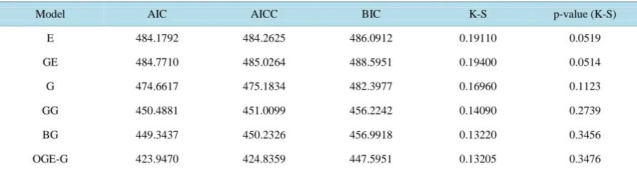
Based on Table 2 and Table 3, it is shown that OGE-G (α, λ, c,β) model is the best among of those distribu-tions because it has the smallest value of (K-S), AIC, CAIC and BIC test.

Substituting the MLE’s of the unknown parameters α, λ, c,β into (32), we get estimation of the variance co-variance matrix as the following

3 7 4 4

7 8 6 6

1

0 4 6 5 4

4 6 4 3

1.5022 10 2.7638 10 1.4405 10 9.6331 10 2.7638 10 4.4773 10 1.7837 10 2.7858 10 1.4405 10 1.7837 10 8.4428 10 1.9127 10 9.6331 10 2.7858 10 1.9127 10 1.5309 10

I

− − − −

−

− − − −

 × × − × × 

 _× _× ₋ _× _× 

 

=

₋ _× ₋ _× _× ₋ _× 

 

× × − × ×

 

The approximate 95% two sided confidence intervals of the unknown parameters α, λ, c and β are

[

0, 0.116

]

,

[

0, 0.001

]

,

[

0.060, 0.096

]

and

[

0.116, 0.270

]

, respectively.

[image:11.595.164.465.211.271.2]

To show that the likelihood equation have unique solution, we plot the profiles of the log-likelihood function of α, λ, β and c in Figure 4 and Figure 5.

Table 1. The data from Aarset [9].

0.1 0.2 1 1 1 1 1 2 3 6 7 11 12 18 18 18 18

18 21 32 36 40 45 46 47 50 55 60 63 63 67 67 67 67

[image:11.595.92.540.344.699.2]

72 75 79 82 82 83 84 84 84 85 85 85 85 85 86 86

Table 2. The MLE’s, log-likelihood for Aarset data.

Model

MLE’s

-L

ˆ

α _βˆ _λˆ cˆ

E 0.0219 - - - 241.0896

GE 0.0212 0.9012 - - 240.3855

G - - 0.00970 0.0203 235.3308

GG - 0.2625 0.00010 0.0828 222.2441

BG 0.2158 0.2467 0.00030 0.0882 220.6714

[image:11.595.90.537.597.717.2]

OGE-G 0.0400 0.1940 0.000345 0.0780 215.9735

Table 3. The AIC, CAIC, BIC and K-S values for Aarset data.

Model AIC AICC BIC K-S p-value (K-S)

E 484.1792 484.2625 486.0912 0.19110 0.0519

GE 484.7710 485.0264 488.5951 0.19400 0.0514

G 474.6617 475.1834 482.3977 0.16960 0.1123

GG 450.4881 451.0099 456.2242 0.14090 0.2739

BG 449.3437 450.2326 456.9918 0.13220 0.3456

(12)

[image:12.595.86.542.75.508.2]

Figure 4. The profile of the log-likelihood function of α, λ.

Figure 5. The profile of the log-likelihood function of c, β.

The nonparametric estimate of the survival function using the Kaplan-Meier method and its fitted parametric estimations when the distribution is assumed to be ED, GED, GD, GGD and OGE-GD are computed and plotted in Figure 6.

Figure 7, gives the form of the hazard rate for the ED, GED, GD, GGD, BGD and OGE-GD which are used to fit the data after replacing the unknown parameters included in each distribution by their MLE.

7. Conclusion

(13)

[image:13.595.186.440.88.277.2]

Figure 6. The Kaplan-Meier estimate of the survival function.

Figure 7. The Fitted hazard rate function for the data.

Acknowledgments

The authors are grateful to the anonymous referee for a careful checking of the details and for helpful comments that improved this paper.

References

[1] Pollard, J.H. and Valkovics, E.J. (1992) The Gompertz Distribution and Its Applications. Genus, 48, 15-28.

[2] Marshall, A.W. and Olkin, I. (2007) Life Distributions. Structure of Nonparametric, Semiparametric and Parametric Families.Springer, New York.

[3] Abu-Zinadah, H.H. and Aloufi, A.S. (2014) Some Characterizations of the Exponentiated Gompertz Distribution. In-ternational Mathematical Forum, 9, 1427-1439.

[4] El-Gohary, A., Alshamrani, A. and Al-Otaibi, A.N. (2013) The Generalized Gompertz Distribution. Applied Mathe-matical Modelling, 37, 13-24. http://dx.doi.org/10.1016/j.apm.2011.05.017

[image:13.595.187.440.296.522.2]

(14)

Statis-tics-Theory and Methods, 31, 497-512. http://dx.doi.org/10.1081/STA-120003130

[6] Jafari, A.A., Tahmasebi, S. and Alizadeh, M. (2014) The Beta-Gompertz Distribution. Revista Colombiana de Esta- dĺstica, 37, 141-158. http://dx.doi.org/10.15446/rce.v37n1.44363

[7] Mudholkar, G.S. and Srivastava, D.K. (1993) Exponentiated Weibull Family for Analyzing Bathtub Failure Data.

IEEE Transactions on Reliability, 42, 299-302. http://dx.doi.org/10.1109/24.229504

[8] Tahir, M.H., Cordeiro, G.M., Alizadeh, M., Mansoor, M., Zubair, M. and Hamedani, G.G. (2015) The Odd Genera-lized Exponential Family of Distributions with Applications. Journal of Statistical Distributions and Applications, 2, 1-28. http://dx.doi.org/10.1186/s40488-014-0024-2

[9] Aarset, M.V. (1987) How to Identify a Bathtub Hazard Rate. IEEE Transactions on Reliability, 36, 106-108.

http://dx.doi.org/10.1109/TR.1987.5222310

[10] Gupta, R.D. and Kundu, D. (2007) Generalized Exponential Distribution: Existing Results and Some Recent Devel-opments. Journal of Statistical Planning and Inference, 137, 3537-3547. http://dx.doi.org/10.1016/j.jspi.2007.03.030

[11] Gupta, R.D. and Kundu, D. (2001) Generalized Exponential Distribution: Different Method of Estimations. Journal of Statistical Computation and Simulation, 69, 315-337. http://dx.doi.org/10.1080/00949650108812098

[12] Lenart, A. (2014) The Moments of the Gompertz Distribution and Maximum Likelihood Estimation of Its Parameters.

Scandinavian Actuarial Journal, 2014, 255-277. http://dx.doi.org/10.1080/03461238.2012.687697

[13] Nadarajah, S. and Kotz, S. (2006) The Beta Exponential Distribution. Reliability Engineering & System Safety, 91, 689-697. http://dx.doi.org/10.1016/j.ress.2005.05.008

[14] Pasupuleti, S.S. and Pathak, P. (2010) Special Form of Gompertz Model and Its Application. Genus, 66, 95-125. [15] Gupta, R.D. and Kundu, D. (1999) Generalized Exponential Distribution. Australian and New Zealand Journal of