Production Decoupling under US Farm Programs

Published Online January 2014 (http://www.scirp.org/journal/nr) http://dx.doi.org/10.4236/nr.2014.51003

Production Decoupling under US Farm Programs

Charles B. Moss

1

, Andrew Schmitz

1

, Troy G. Schmitz

2 1

Food and Resource Economics, IFAS, University of Florida, Gainesville, USA; 2Morrison School of Agribusiness and Resource Management, Arizona State University, Mesa, USA.

Email: [email protected], [email protected], [email protected]

Received September 5th, 2013; revised November 3rd, 2013; accepted December 2nd, 2013

Copyright © 2014 Charles B. Moss et al. This is an open access article distributed under the Creative Commons Attribution License, which permits unrestricted use, distribution, and reproduction in any medium, provided the original work is properly cited. In accor-dance of the Creative Commons Attribution License all Copyrights © 2014 are reserved for SCIRP and the owner of the intellectual property Charles B. Moss et al. All Copyright © 2014 are guarded by law and by SCIRP as a guardian.

ABSTRACT

The loan rate and target price are key ingredients in US farm policy. Empirical models of the effect of US agri-cultural policy are based on different degrees of decoupling between price supports and production. Theoreti-cally, rational producers will make decisions based on the loan rate rather than the target price. Therefore, models which are estimated based on a target price specification could significantly overestimate the distortio-nary impact of policy on resource use and production.

KEYWORDS

Decoupling; Loan Rate; Price Suppression; Target Price

1. Introduction

Historically, agricultural policy in the United States has used several mechanisms to support agricultural income. During the 1950s and 1960s, farm prices were supported using a variety of marketing instruments coupled with acreage allotments. Specifically, the Commodity Credit Corporation made non-recourse loans at a stated loan rate for program crops. Under this program, the farmer could simply forfeit the crop in payment of the loan. This led to the accumulation of a large stock of surplus grain. In the 1970s through the 1980s, the agricultural program shifted slightly. The acreage allotments were changed to base acreages. The Commodity Credit Corporation still main-tained a defacto price floor (and typically accumulated stocks). However, an additional instrument referred to as the deficiency payment was introduced that provided for direct payments based on the difference between a man-dated target price and either the higher of the loan rate or the market price over a stated marketing period. The tar-get price for a basic farm commodity in the United States is established by law as a mechanism to support

agricul-tural income (Schmitz et al. 2010 [1]). The loan rate is

the price floor set in agricultural policy legislation that grew out of the operation of the Commodity Credit Cor-poration, which took commodities as collateral at

the loan rate in its non-recourse loan program (Schmitz et

al. 2010 [1]). The farmer then received a deficiency

payment defined as the difference between the target price and the greater of either the loan rate or the market price times the number of base acres (adjusted for set- aside or mandatory acreage reductions) times program yields. The present value of these deficiency payments formed the basis of the production flexibility contracts or Agricultural Market Transaction Act payments under the FAIR Act and remained in the countercyclical payments in more recent agricultural legislation.

con-tinuum. Nor does the WTO offer any kind of empirical gauge about the degree of decoupling.

2. Past Results

Several studies have empirically modeled the impact of US policy. Schmitz, Schmitz, and Dumas (1997 [2]) es-timate the impact of US cotton policy, assuming that farmers make production decisions based on the target price. Later, Schmitz, Rossi, and Schmitz (2007 [3]) show the empirical results under a loan rate specification. Empirical results by Westcott, Young, and Price (2002 [4]); Anton and Le Mouel (2003 [5]); Goodwin and Mi-shra (2005 [6]); and Lin and Dismukes (2005 [7]) are based on producer supply price expectations that fall be- tween the target price and the loan rate.

To highlight the debate, consider the impact of the US cotton policy, which was the basis for a WTO lawsuit launched by Brazil against the United States (Powell and Schmitz 2005 [8]). The impact depends on several inter-related factors: how input subsidies interact with produc-er price supports, producproduc-er price expectations, and the extent to which price supports are decoupled from pro-duction. Cotton subsidies have a direct impact on world cotton prices, depending on the extent to which price supports are coupled to production (Schmitz, Rossi, and

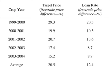
Schmitz 2007 [3]). Table 1 gives the results of the

im-pact of the US cotton policy on world cotton prices under both target price and loan rate specifications. Under the target price specification, the average percentage reduc-tion in world cotton prices over free trade is 20.5 percent for the crops years 1999 through 2004. On the other hand, under the loan rate model, the world cotton price impact is much less at 12.4 percent (Schmitz, Rossi, and Schmitz 2007 [3]).

3. Theoretical Framework

3.1. Production Decisions and Resource Use

The amount of resources used in production generally depends on producer price expectations. In a simple

model framework, consider Figure 1, where S is supply,

Dd is domestic demand, and TD is total demand. If

pro-ducers make decisions at the target price p1 production is

q1. The deficiency payment from the government is

(

p p ba1 2

)

and variable costs total

(

yxq a1

)

.

Suppose instead, producers make production decisions

based on the loan rate p2. Planned production falls to q2.

Variable costs are

(

yxq b₂ ′

)

. Total variable costs are

re-duced by

(

b q q a′ _{2 1}

)

under the loan rate response

mod-el1.

In this formulation, producers gain by making deci

Table 1. Free trade: US cotton target price and loan rate specifications, 1999-2004.

Crop Year

Target Price (freetrade price difference—%)

Loan Rate (freetrade price

difference—%)

1999-2000 29.3 20.5

2000-2001 19.9 10.3

2001-2002 20.7 13.6

2002-2003 17.4 8.7

2003-2004 15.2 8.7

Average 20.5 12.4

[image:2.595.308.538.110.254.2]

Source: Schmitz, Rossi, and Schmitz (2007 [3]).

Figure 1. Target price and loan rate specifications.

sions based on the target price. The net welfare gain

from basing decisions on price p1 rather than price p2 is

(

p p b a1 2 ′

)

in spite of the added variable costs

(

b q q a′ 2 1

)

.

From a resource use standpoint, consider again Figure

1, where p3 represents a price expectation on the part of

producers which is an expected price above the exported

target price p1. At price p3, output is expected to increase

to q3. As comparison, if in the previous year t – 1,

pro-ducers based decisions at the loan rate price p2, then at

time t with a price expectation of p3, variable costs

in-crease by

(

b q q c′ _{2 3}

)

as output increased from q2 to q3.

However, if at time t – 1, the price expectation was the

target price p1, then at time t, the variable costs only

in-creased by

(

aq q c_{1 3}

)

as output only increased from q1 to

q3.

3.2. Loan Rate or Target Price

The question of whether the loan rate or target price af-fects the quantity of a good produced can be traced to the firm’s production decision. Assume that producer choos-es the level of production by determining the level of a single input that maximizes profit expressed as

1_{Note, as shown, that it is possible for an exporter to become an}

[image:2.595.326.518.270.427.2]

( )

Max

t

t t t t x P f x −w x

(1)

where pt is the output price at time t, f x

( )

t is the

stan-dard primal production function given the level of the variable input xt, and wt is the price of the input at time t.

The effect of the loan rate and target price on the quantity supplied is dependent on how each policy variable affects output prices in Equation (1). As a starting point, consid-er the effect of the loan rate which the farmconsid-er receives if the market price is higher than the loan rate. Assuming that the farmer maximizes expected profit, Equation (1) becomes

[

] ( )

Max max ,

t

t t Lt t t t

x E  P P f x −w x (2)

whereE_t

[ ]

. denotes the expectation function given

in-formation available at time t and P_Lt is the loan rate for

the crop at time t. It is trivial to show that expected profit

and level of the variable input increases as the loan rate increases. The debate in the literature involves the effect of the target price.

To develop the effect of the target price we note that the target price is paid on base acres for program or

proven yields. Thus, deficiency payment at time t can be

written as

(

)

(

)

[

]

(

)

1 2 5

1 2 5

, ,

1 max 0, max , , ,

t t t t

t Tt t Lt t t t t

D x x x

P P P y x x x

α − − − − − −   = − _ − _×    (3)

where Dt is the deficiency payment, αt is the set-aside

effective in year t, P_Tt is the target price, and

(

1, 2, 5

)

t t t t

y x − x− x− is the program yield. The

contro-versy on the effect of the target price is dependent on the definition of the program yield. Typically, the farmer could choose to rely on the county average yield or choose to prove another yield based on average historical production. Hence, we represent the program yield as

(

)

5

( )

1 2 5

1

, , max ,

t t t t Ct i t i i

y x₋ x₋ x₋ y a f x₋

=

 

= _{ }



∑



  (4)

where y_Ct is the average crop yield for the county, a_i

is a weight for computing the average program yield (one case would be the use of an Olympic Average to

con-struct program yields; hence the a_i is set to zero for the

high and low yield with the remaining ai =1 3).

Using this formulation for the deficiency payment, the producer’s problem then becomes

[

]

( )

(

1 2 5

)

Max max ,

, ,

t

t t Lt t

x

t t t t t t

E P P f x

w x D x− x− x− 



− +  _. (5)

Under this formulation, the current production deci-sion does not affect the deficiency payment received by the farmer. To capture the effect of production decisions on the deficiency payment, we extend Equation (5) by considering the present value of production decisions

[

]

( )

(

)

(

)

1 1 2 5

, , 0

Max max , , ,

t t

N i

t t Lt t t t t t t t x x

t

E β P P f x w x D x x x

+ ₌ − − −

 _{− +} 

 



∑



  (6)

where

β

=1 1

(

+r

)

is the single period discount rate. Hence, taking the first-order condition of Equation (6) yields

[

] ( )

5

(

)

1 2 5

1

, ,

max , t i t i t i t i t i

t t Lt t i

t t

f x D x x x

E P P w

x β x

+ + − + − + − =  ∂ ∂  − +  _{∂ ∂}  

∑



 _{. (7)}

If we assume that the f x

( )

_t >y_Ct for

( )

*

t t

x N x

∀ ∈ where x_t* is the optimum input level (where

( )

*

t

N x

de-notes an open neighborhood around x*_t), the effect of the deficiency payment on the optimum input level becomes

(

)

[

]

( )

5

1 2 5

1

5 1

, ,

max 0, max , 0

t i t i t i t i i

t

i t

t i

t t i Tt i t i Lt i i

i t

D x x x

E

x

f x

E P P P a

x β β α + + − + − + − = + + + + =  ∂  =  _∂    ∂  _ − _ ≥   _∂

∑

∑



. (8)

Given that max 0,_ P_{Tt i+} −max

[

P_{t i+},P_{Lt i+}

]

_≥0, the supply of output will be greater for Equations (7) and (8) (with deficiency payments) than for Equation (2) (with only the loan rate). However,

[

]

( )

[

]

( )

(

)

(

)

[

]

( )

1 *

1 2 5

, , ₀

Max max ,

Max max , , ,

Max max ,

t

t t

t

t t t Tt t t t

x

N i

t t t Lt t t t t t t t

x x _t

t t t Lt t t t

x

x E P P f x w x

x E P P f x w x D x x x

x E P P f x w x

where x_t is the optimal level of input used when the

farmer realizes the target price (i.e., farmers respond to

the target price directly), x*_t is the optimal level of

in-put used when the farmer realizes returns from the target

price from the deficiency payment over time, and x_t is

the optimal level of input used when the farmer only

re-sponds to the loan rate because 5

1 1

i i i=β a

∑

 .

In the FAIR Act of 1996, the Agricultural Market Transaction Act payments were fixed so that

( )

. 0

t t

D x

∂ ∂ = , implying xt*=xt. While some

adjust-ment in base yield was allowed with the passage of the Farm Security and Rural Investment Act of 2002, the countercyclical payments followed the fixed program yield formulation introduced in 1996.

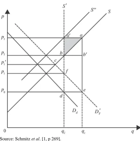
Building on this formulation, Figure 2 illustrates both

the loan rate and target price model for cotton. Domestic

demand is given by D_d and supply is given by S. Under

the loan rate-based decoupled scenario, the equilibrium

price and quantity are p_l and q_l. The coupled loan

deficiency payments (LDPs) to producers equal

(

p p fbl i

)

,

while the decoupled countercyclical payments equal

(

p p bat l ′

)

if producers respond to the loan rate, pl, and

not to the net target price, p_t. The producers gain from

price supports equal

(

p p ba_{t l} ′

)

. The magnitude of these

producer rents for cotton is $1.74 billion for 2002 (Schmitz, Rossi, and Schmitz 2007 [3]).

Now we show the effects if the producers respond to the target price set rather than the loan rate. In the litera-ture there is considerable confusion as to whether far-mers respond to the loan rate, target price, or to some price in between. However, as we show, farmers should make decisions based on the loan rate and not the target

price (Figure 2). Given that the countercyclical payment

is determined by base acres and base yield, the amount of payment is fixed with respect to input decisions. That is,

farmers cannot capture

(

a ba′

)

by responding to the

target price rather than the loan rate. Since the transfer of countercyclical payments from taxpayers to farmers does not affect production, the comparison of the welfare im-pacts under the loan rate and the target price is somewhat trivial.

Consider the effects if producers responded to the tar-get price rather than the loan rate. In this case, producers

would suffer a loss of

(

a ba′

)

. Specifically, if the

pro-ducers attempt to increase production in response to the

target price, they would only receive the loan rate p_l;

hence, they would lose the cost of production on

(

qt−ql

)

units of output. By attempting to respond to

the target price, farmers add the cost

(

bq q_{l t}a

)

. However,

they only receive revenue based on the loan rate

(

bq ql tb′

)

. Since the market price at this additional

quan-tity falls to p₀, the farmer now receives

(

p₀0 eq_t

)

from the market and

(

p pl 0eb′

)

as a loan payment.

[image:4.595.309.536.82.311.2]

Source: Schmitz et al. [1, p 269].

Figure 2. Loan rate model and target price model.

4. Summary and Conclusions

The impact of US agricultural subsidies is increasingly being scrutinized, especially in view of the successful Brazilian challenge to US cotton subsidies in the WTO. The impact of US subsidies can be significant (Powell and Schmitz 2005 [8]), depending on the degree of de-coupling between production and price supports. Farmers’ decisions based on loan rates yield outcomes that are more decoupled than those based on target prices. Our theoretical results show that rational producers will make production decisions based on loan rates. This is impor-tant since a WTO ruling may incorrectly find a high de-gree of policy coupling if they rely on results based on a target price specification when the true empirical results should be grounded on a loan rate phenomenon. The sig-nificant price suppression terminology used in the WTO ruling unfortunately does not provide guidance as to where producers respond to the price continuum in our model. Moreover, the findings in the WTO rulings do not give an empirical gauge as to the degree of decoupling. For example, the impact of US cotton policy on world prices can range from between 20.5 and 12.4 percent, depending on the degree of decoupling assumed in em-pirical specification.

free market setting.

REFERENCES

[1] A. Schmitz, C. B. Moss, T. G. Schmitz, H. W. Furtan, and H. C. Schmitz, “Agricultural Policy, Agribusiness, and Rent-Seeking Behaviour,” 2nd Edition, University of Toronto Press, Toronto, 2010.

[2] T. G. Schmitz, A. Schmitz and C. Dumas, “Gains from Trade, Inefficiency of Government Programs, and the Net Economic Effects of Trading,” Journal of Political Economy, Vol. 105, No. 3, 1997, pp. 637-647.

http://dx.doi.org/10.1086/262086

[3] A. Schmitz, F. Rossi and T. Schmitz, “US Cotton Subsi-dies: Drawing a Fine Line on the Degree of Decoupling,” Journal of Agricultural and Applied Economics, Vol. 39, No. 1, 2007, pp. 135-149.

[4] P. Westcott, C. Young and J. Price, “The 2002 Farm Act: Provisions and Implications for Commodity Markets,” AIB778, USDA/ERS, Washington DC, 2002.

[5] J. Anton and C. Le Mouel, “Do Countercyclical Payments

in the FSRI Act Create Incentives to Produce?” Proceed-ings of the 25th International Conference of Agricultural Economists, Durban, 2003.

http://ageconsearch.umn.edu/bitstream/25811/1/cp03an02 .pdf

[6] B. Goodwin and A. Mishra, “Another Look at Decoupl-ing: Additional Evidence on the Production Effects of Direct Payments,” American Journal of Agricultural Economics, Vol. 87, No. 5, 2005, pp. 1200-1210. http://dx.doi.org/10.1111/j.1467-8276.2005.00808.x

[7] W. Lin and R. Dismukes, “Risk Considerations in Supply Response: Implications for Countercyclical Payments’ Production Impact,” Proceedings of the American Agri-cultural Economics Association Conference, Providence, 2005.

http://ageconsearch.umn.edu/bitstream/19304/1/sp05li09. pdf