DEA Scores’ Confidence Intervals with Past Present and Past Present Future Based Resampling

http://dx.doi.org/10.4236/ajor.2016.62015

DEA Scores’ Confidence Intervals with

Past-Present and Past-Present-Future

Based Resampling

Kaoru Tone

1

, Jamal Ouenniche

2

1_{National Graduate Institute for Policy Studies, Tokyo, Japan} 2_{University of Edinburgh, Business School, Edinburgh, UK}

Received 8 January 2016; accepted 5 March 2016; published 8 March 2016

Copyright © 2016 by authors and Scientific Research Publishing Inc.

This work is licensed under the Creative Commons Attribution International License (CC BY). http://creativecommons.org/licenses/by/4.0/

Abstract

In data envelopment analysis (DEA), input and output values are subject to change for several reasons. Such variations differ in their input/output items and their decision-making units (DMUs). Hence, DEA efficiency scores need to be examined by considering these factors. In this paper, we propose new resampling models based on these variations for gauging the confidence intervals of DEA scores. The first model utilizes past-present data for estimating data variations imposing chronological order weights which are supplied by Lucas series (a variant of Fibonacci series). The second model deals with future prospects. This model aims at forecasting the future efficiency score and its confidence interval for each DMU. We applied our models to a dataset composed of Japanese municipal hospitals.

Keywords

Data Variation, Resampling, Confidence Interval, Past-Present-Future DEA, Hospital

1. Introduction

122

DEA provides a consistent estimator of arbitrary monotone and concave production functions when the (one- sided) deviations from such a production function are degraded as stochastic variations in technical inefficiency. Afterwards the treatment of data variations has taken a variety of forms in DEA. In fact, several authors investi-gated the sensitivity of DEA scores to data variations in inputs and/or outputs using sensitivity analysis and su-per-efficiency analysis. For example, Charnes and Neralić [4] and Neralić [5] used conventional linear pro-gramming-based sensitivity analysis under additive and multiplicative changes in inputs and/or outputs to inves-tigate the conditions under which the efficiency status of an efficient DMU is preserved (i.e., basis remains un-changed), whereas Zhu [6] performed sensitivity analysis using various super-efficiency DEA models in which a test DMU is not included in the reference set. This sensitivity analysis approach simultaneously considers input and output data perturbations in all DMUs, namely, the change of the test DMU and the remaining DMUs. On the other hand, several authors investigated the sensitivity of DEA scores to the estimated efficiency frontier. For example, Simar and Wilson [7] [8] used a bootstrapping method to approximate the sampling distributions of DEA scores and to compute confidence intervals (CIs) for such scores. Barnum et al. [9] provided an alterna-tive methodology based on Panel Data Analysis (PDA) for computing CIs of DEA scores; in sum, they com-plemented Simar and Wilson’s bootstrapping by using panel data along with generalized least squares models to correct CIs for any violations of the standard statistical assumptions (i.e., DEA scores are independent and iden-tically distributed, and normally distributed) such as the presence of contemporaneous correlation, serial correla-tion and heteroskedasticity. Note, however, that [7] and [8] do not take account of data variacorrela-tions in inputs and outputs. Note also that although [9] takes account of data variations in inputs and outputs by considering panel data and computing DEA scores separately for each cross section of the data, the reliability of the approach de-pends on the amount of data available for estimating the generalized least squares models.

In this paper, we follow the principles stated in Cook, Tone and Zhu [10] and believe that DEA performance measures are relative, not absolute, and frontiers-dependent. DEA scores undergo a change depending on the choice of inputs, outputs, DMUs and DEA models by which DMUs are evaluated. In this paper, we compute ef-ficiency scores or equivalently solve the frontier problem using the non-oriented slacks-based super-efef-ficiency model. Our approach deals with variations in both the estimated efficiency frontier and the input and output data directly by resampling from historical data over two different time frames (i.e., past-present and past-present- future); thus, the production possibility set for the entire DMUs differs with every sample1. In addition, our ap-proach works for both small and large sets of data and does not make any parametric assumptions. Hence, our approach presents another alternative for computing confidence intervals of DEA scores.

This paper unfolds as follows. Section 2 presents a generic methodological framework to estimate the confi-dence intervals of DEA scores under a past-present time frame and extends it to the past-present-future time frame. Section 3 presents a healthcare application to illustrate the proposed resampling framework. Finally, sec-tion 5 concludes the paper.

2. Proposed Methodology

In this section, we propose a generic methodological framework to estimate the confidence intervals of DEA scores under a past-present time frame. This framework is generic in that its implementation requires a number of decisions to be made as will be discussed hereafter. Then, we extend the use of this framework to the past- present-future time frame.

2.1. Past-Present Based Framework

The first framework is designed for when past-present information on say m inputs and s outputs of a set of n

DMUs is available; that is,

(

X Yt, t

) (

=

{

xi jt_, ,ytr j_,

)

;i=1,, ,m r=1,, ,s j=1, , ,n

}

t=1,,T , where period T

denote the present and periods 1 though T−1 represent the past. The proposed framework could be summa-rized as follows:

Initialization Step

Choose an appropriate DEA model for computing the efficiency scores of DMUs;

Use the chosen DEA model to estimate the DEA scores of DMUs based on the present information; that is,

1

(

XT,YT

)

. Let

δ

Tj;j=1,,n denote such scores-in the iterative step, we gauge the confidence interval of

; 1, ,

T

j j n

δ

=  using replicas of historical data

(

Xt,Yt

)

,t=1,,T;

Choose an appropriate scheme, say w, to weigh the available information on the past and the present; Choose a confidence level 1−α;

Choose the number of replicas or samples to draw from the past, say B, along with any properties they should satisfy before being considered appropriate to use for generating the sampling distributions of

δ

Tj;j=1,,n and computing their confidence intervals;

Set an indicator variable, say property_status, that reflects whether the B replicas satisfy the required properties or not to false.

Iterative Step

The generic nature of this framework requires a number of decisions to be made for its implementation for a particular application. Hereafter, we shall discuss how one might make such decisions.

2.1.1. Choice of a DEA Model

In principle one might choose from a relatively wide range of DEA models; however, given the nature of this exercise we recommend the use of the non-oriented super slacks-based measure model (Tone [12] and Ouen-niche et al. [13]) under the relevant returns-to-scale (RTS) setup (e.g., constant, variable, increasing, decreasing) as suggested by the RTS analysis of the dataset one is dealing with. This model is an extension of the SBM (slacks-based measure) model of Tone [14]—see also [15]. Although one could use other models (e.g., radial or oriented), our recommendation is based on the following reasons. First, as a non-radial model, the SBM model is appropriate for taking account of input and output slacks which affect efficiency scores directly, whereas the ra-dial models are mainly concerned with the proportional changes in inputs or outputs. Thus, SBM scores are more sensitive to data variations than the radial ones. Second, the non-oriented SBM model can deal with in-put-surpluses and output-shortfalls within the same scheme. Finally, as most DEA scores are bounded by unity (≤1, or ≥1), difficulties in comparing efficient DMUs maybe encountered; therefore, we recommend using the super-efficiency version of the non-oriented SBM as it removes such unity bounds.

2.1.2. Choice of a Weighting Scheme for Past-Present Information

Many different weighting schema could be used to weigh information on the past and the present; that is,

( )

, ; 1, , , 1, , , 1, ,

t i j

x i=  m j=  n t=  T and

( )

t_, ; 1, , , 1, , , 1, ,

r j

y r=  s j=  n t= T. The choice of the weight-ing scheme should reflect the decision makers’ perspective and knowledge of the application area on how the past should influence the present. In this paper, we set the weight w_t of a period t so that the weights are in-creasing in t; in sum, we assume that more recent periods carry information that is more relevant to estimate ef-ficiency scores in the present time. Thus, the following Lucas number series

(

l₁,,l_T

)

, a variant of Fibonacci series, is a candidate where lt+₂= +lt lt+₁;t=1,,T−2,l₁=1,l₂=2. Let L denote the sum of the series:

1

T t t

2 0.1053

w = , w₃=0.1579, w₄=0.2631, and w₅=0.4211. Thus, the influence of the past periods fades away gradually as we approach the present.

2.1.3. Choice of the Replication Process and the Number of Replicas

In this paper, we regard historical data

(

X Yt, t

) (

=

{

xi jt_, ,yr jt_,

)

;i=1,, ,m r=1,, ,s j=1,, , ,n

}

t=1,,T as

discrete events with probability w_t and cumulative probability

1 ; 1, ,

t

t k k

W =

∑

₌ w t=  T. We propose a repli- cation process based on bootstrapping. First proposed by Efron [16], nowadays bootstrapping refers to a collec-tion of methods that randomly resample with replacement from the original sample. Thus, in bootstrapping, the population is to the sample what the sample is to the bootstrapped sample. Bootstrapping could be either para-metric or non-parapara-metric. Parapara-metric bootstrapping is concerned with fitting a parapara-metric model, which in our case would be a theoretical distribution, to the data and sampling from such fitted distribution. This is a viable approach for large datasets where the distribution of each input and each output could be reasonably approxi-mated by a specific theoretical distribution. However, when no theoretical distribution could serve as a good ap-proximation to the empirical one or when the dataset is small, non-parametric bootstrapping is the way to pro-ceed. Non-parametric bootstrapping does not make any assumptions except that the sample distribution is a good approximation to the population distribution, or equivalently the sample is representative of the population. Consequently, datasets with different features require different resampling methods that take account of such features and thus generate representative replicas.

For a non-correlated and homoskedastic dataset, one could for example use smooth bootstrapping or Bayesian bootstrapping, where smooth bootstrapping generates replicas by adding small amounts of zero-centered random noise (usually normally distributed) to resampled observations, whereas Bayesian bootstrapping generates rep-licas by reweighting the initial data set according to a randomly generated weighting scheme. In this paper, we recommend the use of a variant of Bayesian bootstrapping whereby the weighting scheme consists of the Lucas number series-based weights w_t presented above, because it is more appropriate when one is resampling over a past-present time frame and more recent information is considered more valuable. For a non-correlated and ho-moskedastic dataset, our Data Generation Process (DGP) may be summarized as follows. First, a random num-ber ρ is drawn from the uniform distribution over the interval [0,1], then whichever cross section data

(

X Yt, t

)

so that W_t−₁< ≤ρ W_t is resampled, where W0=0. This process is repeated as many times as neces-sary to produce the required number of valid replicas or samples.

On the other hand, for a correlated and/or heteroskedastic dataset, one could use one of the block bootstrap-ping methods, where replicas are generated by splitting the dataset into non-overlapbootstrap-ping blocks (simple block bootstrap) or into overlapping blocks of the same or different lengths (moving block bootstrap), sampling such blocks with replacement and then aligning them in the order they were drawn. The main idea of all block boot-strap procedures consists of dividing the data into blocks of consecutive observations of length , say

(

) (

1 1

) (

1 1

)

, , , , , ,

t t t t t t

X Y X + Y + X + − Y + −

 

    , and sampling the blocks randomly with replacement from all possible Blocks—for an overview of bootstrapping methods, the reader is referred to [17]. The block bootstrap procedure with blocks of non-random length can be summarized as follows:

Input:Block length ∈ so that  T .

Step 1: Draw randomly and independently block labels, say b b₁, ₂,,bR+₁, from the set of labels, say L,

where R=

[ ]

T  , L=

{

1,+1, 2+1,,

(

R−1

)

+1

}

if non-overlapping blocks are considered, and

{

1, 2, , 1

}

L=  T− + if overlapping blocks are considered.

Step 2: Lay the blocks 

(

_Xbk,_Ybk

) (

, _Xbk+1,_Ybk+1

) (

, , _Xbk+ −1,_Ybk+ −1

)

;_k=1, ,_R+1

      , end-to-end in the or-

der sampled together and discard the last − +T R observations to form a bootstrap series

(

_ˆ1 _ˆ1

) (

_ˆ2 _ˆ2

) (

_{ˆ ˆ}

)

, , , , , T, T

X Y X Y  X Y .

Output:Bootstrap sample

(

X Yˆ1,ˆ1

) (

, Xˆ2,Yˆ2

) (

,, XˆT,YˆT

)

.

2.1.4. Choice of the Properties the Replicas Should Satisfy

As replicas are required to be representative of the dataset under consideration, one would have to perform a preliminary analysis of the data to find out about its features; namely, whether it is correlated or not and whether it is heteroskedastic or not using statistical tests such as the ones used in [9]. For a correlated and/or heteroske-dastic dataset, the same relevant statistical tests would have to be used to find out whether the replicas are rep-resentative or not. When replicas are not reprep-resentative, one would have to reject them and resample again. However, for a non-correlated and homoskedastic dataset, one could use hypothesis tests or confidence intervals based on Fisher’s z transformation to compare correlation patterns in past and present data. For example, for the present time period data, one could compute the correlation coefficient between all pairs of inputs, outputs, and input-output over all DMUs. Then, compute their ζ% confidence intervals; e.g., 95%, using Fisher’s z transfor-mation [18]. If the corresponding correlation of a resampled data is out of range of this interval, we discard this resample data. Thus, inappropriate samples with unbalanced inputs and outputs relative to the inputs and outputs of the last period are excluded from resampling. The above noted 95% confidence interval is not compulsory. The narrower the interval, the closer the resample will be to the last period data.

2.2. Past-Present-Future Time Based Framework

In the previous subsection, we utilized historical data

(

_{X Y}t, t

)

,_t=1,_,_{T to gauge the confidence interval of} the last period’s scores. In this section, we forecast the “future”; namely,

(

XT+1,YT+1

)

by using “past-present” data

(

_{X Y}t, t

)

,_t=1,_,_{T and forecast the efficiency scores of the future DMUs along with their confidence} in-tervals. In order to avoid repetition, hereafter we shall discuss how the past-present time based framework could be extended to the past-present-future context. First, we have to forecast the future; to be more specific, given the observed historical data

(

x_{i j}t_, ,y_{r j}t_,

)

,t=1,,T for a certain input i i

(

=1,,m

)

and output r r

(

=1,,s

)

of a DMU j j

(

=1,,n

)

, we wish to forecast

(

1 1

)

, , ,

T T i j r j

x + y + . There are several forecasting engines available for this purpose. Once these forecasts are obtained, we then estimate the super-efficiency score of the “future” DMU

(

_XT+1_,YT+1

)

_{using the non-oriented super slacks-based measure model. Finally, given the past-present-}

future inter-temporal data set

(

X Yt, t

)

,t=1,,T+1, we apply the resampling scheme proposed in the previous section and obtain confidence intervals.

3. An Application in Healthcare

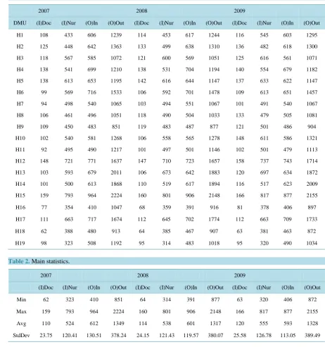
In this study we utilize a dataset concerning nineteen Japanese municipal hospitals from 2007 to 2009 to illus-trate how the proposed framework works. There are approximately 1000 municipal hospitals in Japan and there is large heterogeneity amongst them. We selected nineteen municipal hospitals with more than 400 beds. There-fore, this sample may represent larger acute-care hospitals with homogeneous functions. The data were collected from the Annual Databook of Local Public Enterprises published by the Ministry of Internal Affairs and Com-munications. For illustration purposes, we chose for this study two inputs; namely, Doctor ((I)Doc) and Nurse ((I)Nur), and two outputs; namely, Inpatient ((O)In) and Outpatient ((O)Out). Table 1 exhibits the data, while

[image:6.595.75.538.95.589.2]

Table 1. The data.

2007 2008 2009

DMU (I)Doc (I)Nur (O)In (O)Out (I)Doc (I)Nur (O)In (O)Out (I)Doc (I)Nur (O)In (O)Out

H1 108 433 606 1239 114 453 617 1244 116 545 603 1295

H2 125 448 642 1363 133 499 638 1310 136 482 618 1300

H3 118 567 585 1072 121 600 569 1051 125 616 561 1071

H4 138 541 699 1210 138 531 704 1194 140 554 679 1182

H5 138 613 653 1195 142 616 644 1147 137 633 622 1147

H6 99 569 716 1533 106 592 701 1478 109 613 651 1457

H7 94 498 540 1065 103 494 551 1067 101 491 540 1067

H8 106 461 496 1051 118 490 504 1033 133 479 505 1081

H9 109 450 483 851 119 483 487 877 121 501 486 904

H10 102 540 581 1268 106 558 565 1278 148 611 586 1321

H11 92 495 490 1217 101 497 501 1146 102 501 479 1113

H12 148 721 771 1637 147 710 723 1657 158 737 743 1714

H13 103 593 679 2011 106 673 642 1883 120 697 634 1872

H14 101 500 613 1868 110 519 617 1894 116 517 623 2009

H15 159 793 964 2224 160 801 906 2148 166 817 877 2155

H16 77 354 410 1047 68 359 391 916 81 378 406 897

H17 111 663 717 1674 112 645 702 1774 112 663 709 1733

H18 62 388 480 913 64 385 467 907 63 381 463 872

H19 98 323 508 1192 95 314 483 1018 95 320 490 1034

Table 2. Main statistics.

2007 2008 2009

(I)Doc (I)Nur (O)In (O)Out (I)Doc (I)Nur (O)In (O)Out (I)Doc (I)Nur (O)In (O)Out

Min 62 323 410 851 64 314 391 877 63 320 406 872

Max 159 793 964 2224 160 801 906 2148 166 817 877 2155

Avg 110 524 612 1349 114 538 601 1317 120 555 593 1328

StdDev 23.75 120.41 130.51 378.24 24.15 121.43 119.57 380.07 25.58 126.78 113.05 389.49

3.1. Illustration of the Past-Present Framework

We applied the proposed procedure to the historical data of nineteen hospitals for the two years 2008-2009 in

Table 1. We excluded the year 2007 data, because they belong to a different population than 2009 as explained in Preliminary results (Panel). Note that historical data may suffer from accidental or exceptional events, for example, oil shock, earthquake, financial crisis, environmental system change and so forth. We must exclude these from the data. If some data are under age depreciation, we must adjust them properly. In this study, we use Lucas weights for past and present data. However, we can use other weighting schema (e.g., exponential) as well.

[image:7.595.89.533.380.714.2]

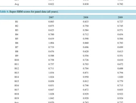
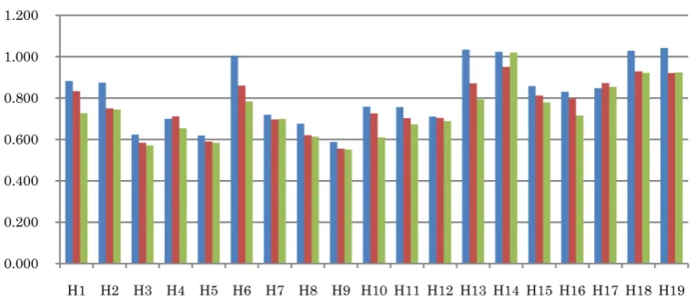
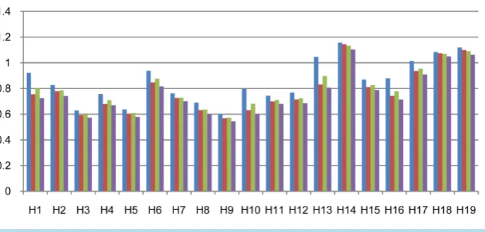
Table 3. Super-SBM scores by cross section (year).

2007 2008 2009

H1 0.883 0.905 0.754

H2 0.875 0.801 0.779

H3 0.623 0.615 0.592

H4 0.700 0.765 0.680

H5 0.619 0.620 0.604

H6 1.004 0.942 0.848

H7 0.719 0.732 0.725

H8 0.676 0.651 0.631

H9 0.588 0.583 0.568

H10 0.758 0.764 0.631

H11 0.757 0.740 0.698

H12 0.711 0.741 0.714

H13 1.034 1.025 0.831

H14 1.039 1.107 1.145

H15 0.858 0.857 0.811

H16 0.831 0.847 0.742

H17 0.847 0.948 0.937

H18 1.034 1.050 1.074

H19 1.071 1.072 1.100

Avg 0.822 0.830 0.782

Table 4. Super-SBM scores for panel data (all years).

2007 2008 2009

H1 0.883 0.833 0.727

H2 0.875 0.750 0.745

H3 0.623 0.584 0.571

H4 0.700 0.712 0.654

H5 0.619 0.590 0.584

H6 1.004 0.860 0.783

H7 0.719 0.696 0.699

H8 0.676 0.620 0.613

H9 0.588 0.556 0.551

H10 0.758 0.726 0.610

H11 0.757 0.703 0.672

H12 0.711 0.704 0.688

H13 1.034 0.871 0.794

H14 1.024 0.950 1.020

H15 0.858 0.812 0.779

H16 0.831 0.798 0.715

H17 0.847 0.872 0.855

H18 1.028 0.929 0.922

H19 1.042 0.920 0.924

[image:8.595.78.538.76.511.2]

Table 5. Correlation matrix.

Doc Nurse Inpatient Outpatient

Doc 1 0.7453 0.7372 0.5178

Nurse 0.7453 1 0.8610 0.7387

Inpatient 0.7372 0.8610 1 0.8264

Outpatient 0.5178 0.7387 0.8264 1

Table 6. Fisher 95% confidence lower/upper bounds for correlation matrix.

Lower bounds

Doc Nurse Inpatient Outpatient

Doc 0.4400 0.4255 0.0832

Upper Nurse 0.8961 0.6681 0.4281

bounds Inpatient 0.8926 0.9455 0.5959

[image:8.595.117.509.237.479.2]

Outpatient 0.7869 0.8932 0.9311

Figure 1. Super-SBM scores by cross section (year).

[image:8.595.123.506.534.699.2]

[image:9.595.87.537.278.377.2]

0.5178 and its 95% lower/upper bounds are respectively 0.0832 and 0.7869. In addition, we report Fisher 20% confidence lower/upper bounds in Table 7. The intervals are considerably narrowed down compared with Fisher 95% case.

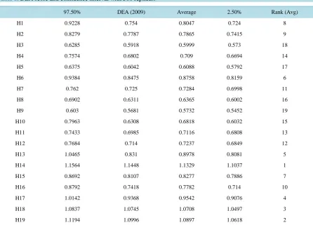
Table 8 exhibits results obtained by 500 replicas where the column DEA is the last period’s (2009) efficiency score and Average indicates the average score over 500 replicas. The column Rank is the ranking of average scores. We applied Fisher 95% threshold and found no out-of-range samples. Figure 3 shows the 95% confi-dence intervals for the last period’s (2009) DEA scores along with Average scores. The average of the 95% con-fidence interval for all hospitals is 0.10.

In the Fisher 95% (ζ95) case, we found no discarded samples, whereas in the Fisher 20% (ζ20) case, 1945 samples were discarded before getting 500 replicas. Table 9 shows the comparisons of scores calculated by both thresholds, where we cannot see significant differences.

Note that one resample produces one efficiency score for each DMU. We compared 500 and 5000 replicas and obtained the 95% confidence interval as exhibited in Table 10. As can be seen, the difference is negligibly small. 500 replicas may be acceptable in this case. However, the number of replicas depends on the numbers of

Table 7. Fisher 20% confidence lower/upper bounds for correlation matrix.

Lower bounds

Doc Nurse Inpatient Outpatient

Doc - 0.71578 0.70695 0.46998

Upper Nurse 0.77214 - 0.8437 0.70854

bounds Inpatient 0.76482 0.87652 - 0.80525

[image:9.595.91.538.395.716.2]

Outpatient 0.56266 0.76614 0.84547 -

Table 8. DEA score and confidence interval with 500 replicas.

97.50% DEA (2009) Average 2.50% Rank (Avg)

H1 0.9228 0.754 0.8047 0.724 8

H2 0.8279 0.7787 0.7865 0.7415 9

H3 0.6285 0.5918 0.5999 0.573 18

H4 0.7574 0.6802 0.709 0.6694 14

H5 0.6375 0.6042 0.6088 0.5792 17

H6 0.9384 0.8475 0.8758 0.8159 6

H7 0.762 0.725 0.7284 0.6998 11

H8 0.6902 0.6311 0.6365 0.6002 16

H9 0.603 0.5681 0.5732 0.5452 19

H10 0.7963 0.6308 0.6818 0.6032 15

H11 0.7433 0.6985 0.7116 0.6808 13

H12 0.7684 0.714 0.7237 0.6849 12

H13 1.0465 0.831 0.8978 0.8081 5

H14 1.1564 1.1448 1.1329 1.1037 1

H15 0.8692 0.8107 0.8277 0.7886 7

H16 0.8792 0.7418 0.7782 0.714 10

H17 1.0142 0.9368 0.9542 0.9076 4

H18 1.0837 1.0745 1.0708 1.0497 3

[image:10.595.82.539.100.387.2]

Table 9. Comparisons of Fisher’s 20% (ζ20) and 95% (ζ95) thresholds. ζ20 - ζ95 ζ20 - ζ95

ζ20 97.50% DEA 2.50% ζ95 97.50% DEA 2.50% 97.50% 2.50%

H1 0.9061 0.754 0.724 H1 0.9228 0.754 0.724 −0.017 0.000

H2 0.8247 0.7787 0.7419 H2 0.8279 0.7787 0.7415 −0.003 0.000

H3 0.6279 0.5918 0.5757 H3 0.6285 0.5918 0.573 −0.001 0.003

H4 0.7476 0.6802 0.6684 H4 0.7574 0.6802 0.6694 −0.010 −0.001

H5 0.6375 0.6042 0.5832 H5 0.6375 0.6042 0.5792 0.000 0.004

H6 0.9382 0.8475 0.8168 H6 0.9384 0.8475 0.8159 0.000 0.001

H7 0.7611 0.725 0.6989 H7 0.762 0.725 0.6998 −0.001 −0.001

H8 0.6905 0.6311 0.6011 H8 0.6902 0.6311 0.6002 0.000 0.001

H9 0.6023 0.5681 0.5467 H9 0.603 0.5681 0.5452 −0.001 0.001

H10 0.7903 0.6308 0.6044 H10 0.7963 0.6308 0.6032 −0.006 0.001

H11 0.7469 0.6985 0.6808 H11 0.7433 0.6985 0.6808 0.004 0.000

H12 0.767 0.714 0.6828 H12 0.7684 0.714 0.6849 −0.001 −0.002

H13 1.0445 0.831 0.8081 H13 1.0465 0.831 0.8081 −0.002 0.000

H14 1.1568 1.1448 1.1041 H14 1.1564 1.1448 1.1037 0.000 0.000

H15 0.867 0.8107 0.7886 H15 0.8692 0.8107 0.7886 −0.002 0.000

H16 0.8747 0.7418 0.7222 H16 0.8792 0.7418 0.714 −0.004 0.008

H17 1.0121 0.9368 0.9058 H17 1.0142 0.9368 0.9076 −0.002 −0.002

H18 1.0837 1.0745 1.0491 H18 1.0837 1.0745 1.0497 0.000 −0.001

H19 1.1195 1.0996 1.063 H19 1.1194 1.0996 1.0618 0.000 0.001

Table 10. Comparisons of 5000 and 500 replicas (Fisher 95%).

500 Replica 5000 Replica Difference

500 97.50% DEA 2.50% 5000 97.50% DEA 2.50% 97.50% 2.50%

H1 0.9228 0.754 0.724 H1 0.9184 0.754 0.7227 0.0044 0.0013

H2 0.8279 0.7787 0.7415 H2 0.8266 0.7787 0.7412 0.0013 0.0003

H3 0.6285 0.5918 0.573 H3 0.6291 0.5918 0.5719 −0.0006 0.0011

H4 0.7574 0.6802 0.6694 H4 0.7581 0.6802 0.6679 −0.0007 0.0015

H5 0.6375 0.6042 0.5792 H5 0.6379 0.6042 0.5801 −0.0004 −0.0009

H6 0.9384 0.8475 0.8159 H6 0.9423 0.8475 0.8164 −0.0039 −0.0005

H7 0.762 0.725 0.6998 H7 0.7615 0.725 0.6985 0.0005 0.0013

H8 0.6902 0.6311 0.6002 H8 0.6907 0.6311 0.5998 −0.0005 0.0004

H9 0.603 0.5681 0.5452 H9 0.603 0.5681 0.5456 0 −0.0004

H10 0.7963 0.6308 0.6032 H10 0.7942 0.6308 0.6055 0.0021 −0.0023

H11 0.7433 0.6985 0.6808 H11 0.7447 0.6985 0.6808 −0.0014 0

H12 0.7684 0.714 0.6849 H12 0.7684 0.714 0.6828 0 0.0021

H13 1.0465 0.831 0.8081 H13 1.046 0.831 0.8081 0.0005 0

H14 1.1564 1.1448 1.1037 H14 1.1565 1.1448 1.1026 −1E−04 0.0011

H15 0.8692 0.8107 0.7886 H15 0.8726 0.8107 0.7886 −0.0034 0

H16 0.8792 0.7418 0.714 H16 0.8785 0.7418 0.7198 0.0007 −0.0058

H17 1.0142 0.9368 0.9076 H17 1.0141 0.9368 0.9051 1E−04 0.0025

H18 1.0837 1.0745 1.0497 H18 1.0837 1.0745 1.0459 0 0.0038

H19 1.1194 1.0996 1.0618 H19 1.1193 1.0996 1.0618 1E−04 0

Max 0.0044 0.0038

[image:10.595.89.537.401.718.2]

[image:11.595.145.488.104.268.2]

Figure 3. 95% confidence interval.

inputs, outputs and DMUs. Hence, we need to check the variations of scores by increasing the number of repli-cas.

As to the comparisons of individual hospitals, looking at Hospitals 1 and 2 in Table 8 and Figure 3, we are puzzled which hospital exhibits better performance. Actually, the 2009 score and the Average score are reversed (H1-2009 = 0.754, H1-Average = 0.8047, H2-2009 = 0.7789, H2-Average = 0.7865) and confidence intervals are overlapped. We applied the Wilcoxon rank-sum test and found that Hospital 1 outperforms Hospital 2 at the significant level 1%. In this way, we can compare individual hospitals in efficiency measurements.

Finally, we would like to draw the reader’s attention to the fact that, in some applications, one might set weights to inputs and outputs. Actually, if costs for inputs and incomes from outputs are available, we can evaluate the comparative cost performance of DMUs. In the absence of such information, instead, we can set weights to inputs and outputs. For example, the weights to Doc and Nurse are assumed to be 5 to 1 (on average), and those of Outpatient to Inpatient are 1 to 10 (on average). We can solve this problem via the Weighted-SBM model, which will enhance the reliability and applicability of our approach.

3.2. Illustration of the Past-Present-Future Framework

Hereafter, we shall present numerical results for the past-resent-future framework. In this case we regard 2007- 2008 as the past-present and 2009 as the future. In our application, we used three simple prediction models to forecast the future; namely, a linear trend analysis model, a weighted average model with Lucas weights, and a hybrid model that consists of averaging their predictions.

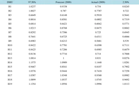
Table 11 reports the forecasts for 2009 obtained by the linear trend analysis model. Table 12 shows the fore-cast DEA score and confidence interval along with the actual super-SBM score for 2009. Figure 4 exhibits 97.5% percent, 2.5% percent, forecast score and actual score. It is observed that, of the nineteen hospitals, the actual 2009 scores of sixteen are included in the 95% confidence interval. The average of Forecast-Actual over the nineteen hospitals was 0.063 (6.3%).

Table 13 reports 2009 forecasts by the weighted average model with Lucas weights and Table 14 shows the

actuals and the forecasts of 2009 scores along with confidence intervals. In this case, only four hospitals are in-cluded in the 95% confidence interval. The average of Forecast-Actual over the nineteen hospitals was 0.056 (5.6%). Although we did not report the results by the Average of Trend and Lucas case, the results are similar to the Lucas case. We compare the number of fails for the three forecast models that actual score is out of 97.5% and 2.5% interval. We have results as exhibited in Table 15. “Trend” gives the best performance among the three in this example.

4. Conclusion

[image:12.595.90.538.443.719.2]

Table 11. 2009 forecasts: linear trend model.

DMU (I)Doc (I)Nurse (O)Inpatient (O)Outpatient

H1 120 473 628 1249

H2 141 550 634 1257

H3 124 633 553 1030

H4 138 521 709 1178

H5 146 619 635 1099

H6 113 615 686 1423

H7 112 490 562 1069

H8 130 519 512 1015

H9 129 516 491 903

H10 110 576 549 1288

H11 110 499 512 1075

H12 146 699 675 1677

H13 109 753 605 1755

H14 119 538 621 1920

H15 161 809 848 2072

H16 59 364 372 785

H17 113 627 687 1874

H18 66 382 454 901

H19 92 305 458 844

Table 12. Forecast DEA score, actual (2009) score and confidence interval: forecast by linear trend model.

DMU 97.50% Forecast (2009) Actual (2009) 2.50%

H1 1.0237 0.9338 0.754 0.8245

H2 1.0027 0.787 0.7787 0.722

H3 0.6649 0.6148 0.5918 0.5641

H4 0.8816 0.8581 0.6802 0.7319

H5 0.6814 0.6421 0.6042 0.5771

H6 1.0213 0.8768 0.8475 0.8062

H7 0.8292 0.7586 0.725 0.6945

H8 0.7641 0.6725 0.6311 0.6066

H9 0.6983 0.6213 0.5681 0.539

H10 0.8422 0.7781 0.6308 0.7111

H11 0.8425 0.7206 0.6985 0.6679

H12 0.8136 0.7716 0.714 0.7068

H13 1.0814 1 0.831 0.8276

H14 1.1575 1.0909 1.1448 1.0281

H15 0.9467 0.8541 0.8107 0.7902

H16 1.0376 0.9444 0.7418 0.7258

H17 1.0387 1.0348 0.9368 0.8982

H18 1.0899 1.0537 1.0745 0.9692

[image:13.595.87.539.101.409.2]

Table 13. 2009 forecasts: Lucas weighted average model.

DMU (I)Doc (I)Nurse (O)Inpatient (O)Outpatient

H1 112 446 613 1242

H2 130 482 639 1328

H3 120 589 574 1058

H4 138 534 702 1199

H5 141 615 647 1163

H6 104 584 706 1496

H7 100 495 547 1066

H8 114 480 501 1039

H9 116 472 486 868

H10 105 552 570 1275

H11 98 496 497 1170

H12 147 714 739 1650

H13 105 646 654 1926

H14 107 513 616 1885

H15 160 798 925 2173

H16 71 357 397 960

H17 112 651 707 1741

H18 63 386 471 909

H19 96 317 491 1076

Table 14. DEA score and confidence interval forecasts: Lucas weighted average model.

97.50% Forecast (2009) Actual (2009) 2.50%

H1 1.0001 0.8974 0.754 0.8469

H2 0.9329 0.8527 0.7787 0.797

H3 0.6448 0.6218 0.5918 0.5987

H4 0.7855 0.7618 0.6802 0.7303

H5 0.6584 0.64 0.6042 0.62

H6 1.0101 0.9604 0.8475 0.9123

H7 0.7813 0.7347 0.725 0.7006

H8 0.7201 0.6867 0.6311 0.6596

H9 0.6578 0.6177 0.5681 0.5894

H10 0.8109 0.7829 0.6308 0.7441

H11 0.8101 0.7573 0.6985 0.7171

H12 0.7623 0.7336 0.714 0.712

H13 1.059 1.0286 0.831 1

H14 1.1306 1.0868 1.1448 1.0409

H15 0.912 0.8665 0.8107 0.8263

H16 0.9296 0.8488 0.7418 0.7869

H17 0.9731 0.9427 0.9368 0.8984

H18 1.0686 1.0443 1.0745 1.0115

[image:13.595.87.540.427.723.2]

[image:14.595.71.542.86.341.2]

Table 15. Number of fails.

Trend Lucas Average of Trend and Lucas

No. of fails 3 15 15

Figure 4. Confidence interval, forecast score and actual 2009 score: forecast by linear trend model.

of DMUs and propose a plan to improve the inputs/outputs of inefficient DMUs. This function is difficult to achieve with similar models in statistics, e.g., stochastic frontier analysis. DEA scores are not absolute but rela-tive. They depend on the choice of inputs, outputs and DMUs as well as on the choice of model for assessing DMUs. DEA scores are subject to change and thus data variations in DEA should be taken into account. This subject should be discussed from the perspective of the itemized input/output variations. From this point of view, we have proposed two models. The first model utilizes historical data for the data generation process, and hence this model resamples data from a discrete distribution. It is expected that, if the historical data are volatile widely, confidence intervals will prove to be very wide, even when the Lucas weights are decreasing depending on the past-present periods. In such cases, application of the moving-average method is recommended. Rolling simulations will be useful for deciding on the choice of the length of the historical span. However, too many past year data are not recommended, because environments, such as healthcare service systems, are changing rapidly. The second model aims to forecast the future efficiency and its confidence interval. For forecasting, we used three models; namely, the linear trend model, the weighted average, and their average. On this subject, Xu and Ouenniche [19] [20] will be useful for the selection of forecasting models, and Chang et al. [21] will provide useful information on the estimation of the pessimistic and optimistic probabilities of the forecast of future in-put/output values.

References

[1] Charnes, A., Cooper, W.W. and Rhodes, E. (1978) Measuring the Efficiency of Decision Making Units. European

Journal of Operational Research, 2, 429-444. http://dx.doi.org/10.1016/0377-2217(78)90138-8

[2] Banker, R. (1993) Maximum Likelihood, Consistency and Data Envelopment Analysis: A Statistical Foundation.

Management Science, 39, 1265-1273. http://dx.doi.org/10.1287/mnsc.39.10.1265

[3] Banker, R. and Natarajan, R. (2004) Chapter 11. Statistical Test Based on DEA Efficiency Scores. In: Cooper, Seiford and Zhu, Eds., Handbook on Data Envelopment Analysis, Springer, 299-321.

http://dx.doi.org/10.1007/1-4020-7798-x_11

[4] Charnes, A and Neralić, L. (1990) Sensitivity Analysis of the Additive Model in Data Envelopment Analysis.

Euro-pean Journal of Operational Research, 48, 332-341. http://dx.doi.org/10.1016/0377-2217(90)90416-9

[6] Zhu, J. (2001) Super-Efficiency and DEA Sensitivity Analysis. European Journal of Operational Research, 129, 443-455. http://dx.doi.org/10.1016/S0377-2217(99)00433-6

[7] Simar, L. and Wilson, P. (1998) Sensitivity of Efficiency Scores: How to Bootstrap in Nonparametric Frontier Models.

Management Science, 44, 49-61. http://dx.doi.org/10.1287/mnsc.44.1.49

[8] Simar, L. and Wilson, P.W. (2000) A General Methodology for Bootstrapping in Non-Parametric Frontier Models.

Journal of Applied Statistics, 27, 779-802. http://dx.doi.org/10.1080/02664760050081951

[9] Barnum, D.T., Gleason, J.M., Karlaftis, M.G., Schumock, G.T., Shields, K.L., Tandon, S. and Walton, S.M. (2011) Es-timating DEA Confidence Intervals with Statistical Panel Data Analysis. Journal of Applied Statistics, 39, 815-828. http://dx.doi.org/10.1080/02664763.2011.620948

[10] Cook, W.D., Tone, K. and Zhu, J. (2014) Data Envelopment Analysis: Prior to Choosing a Model. Omega, 44, 1-4. http://dx.doi.org/10.1016/j.omega.2013.09.004

[11] Yang, M., Wan, G. and Zheng, E. (2014) A Predictive DEA Model for Outlier Detection. Journal of Management

Analytics, 1, 20-41. http://dx.doi.org/10.1080/23270012.2014.889911

[12] Tone, K. (2002) A Slacks-Based Measure of Super-Efficiency in Data Envelopment Analysis. European Journal of

Operational Research, 143, 32-41. http://dx.doi.org/10.1016/S0377-2217(01)00324-1

[13] Ouenniche, J., Xu, B. and Tone, K. (2014) Relative Performance Evaluation of Competing Crude oil Prices’ Volatility Forecasting Models: A Slacks-Based Super-Efficiency DEA Model. American Journal of Operations Research, 4, 235-245. http://dx.doi.org/10.4236/ajor.2014.44023

[14] Tone, K. (2001) A Slacks-Based Measure of Efficiency in Data Envelopment Analysis. European Journal of

Opera-tional Research, 130, 498-509. http://dx.doi.org/10.1016/S0377-2217(99)00407-5

[15] Cooper, W.W., Seiford, L.M. and Tone, K. (2007) Data Envelopment Analysis: A Comprehensive Text with Models, Applications, References and DEA-Solver Software. 2nd Edition, Springer, New York.

[16] Efron, B. (1979) Bootstrap Methods: Another Look at the Jackknife. Annals of Statistics, 7, 1-26. http://dx.doi.org/10.1214/aos/1176344552

[17] Efron B. and Tibshirani R. (1993) An Introduction to the Bootstrap. New York: Chapman & Hall, CRC Press. http://dx.doi.org/10.1007/978-1-4899-4541-9

[18] Fisher, R.A. (1915) Frequency Distribution of the Values of the Correlation Coefficient in Samples from an Indefinite-ly Large Population. Biometrika, 10, 507-521. http://dx.doi.org/10.2307/2331838

[19] Xu, B. and Ouenniche, J. (2011) A Multidimensional Framework for Performance Evaluation of Forecasting Models: Context-Dependent DEA. Applied Financial Economics, 21, 1873-1890.

http://dx.doi.org/10.1080/09603107.2011.597722

[20] Xu, B. and Ouenniche, J. (2012) A Data Envelopment Analysis-Based Framework for the Relative Performance Evaluation of Competing Crude oil Prices’ Volatility Forecasting Model. Energy Economics, 34, 576-583.

http://dx.doi.org/10.1016/j.eneco.2011.12.005

[21] Chang, T.S., Tone, K. and Wu, C.H. (2014) Past-Present-Future Intertemporal DEA Models. Journal of the