Consequences for option pricing of a long memory in volatility

Lancaster University Management School

Working Paper

2001/017

Consequences for Option Pricing of a Long Memory in

Volatility

Stephen John Taylor

The Department of Accounting and Finance Lancaster University Management School

Lancaster LA1 4YX UK

©Stephen John Taylor

All rights reserved. Short sections of text, not to exceed two paragraphs, may be quoted without explicit permission,

provided that full acknowledgement is given.

Stephen J Taylor

Department of Accounting and Finance, Lancaster University, England LA1 4YX

December 2000

Abstract

The economic consequences of a long memory assumption about volatility are

documented, by comparing implied volatilities for option prices obtained from short

and long memory volatility processes. Numerical results are given for options on the

S & P 100 index from 1984 to 1998, with lives up to two years. The long memory

assumption is found to have a significant impact upon the term structure of implied

volatilities and a relatively minor impact upon smile effects. These conclusions are

important because evidence for long memory in volatility has been found in the prices

of many assets.

* S.Taylor@lancaster.ac.uk, www.lancs.ac.uk/staff/afasjt. The author acknowledges the

support of Inquire Europe, with particular thanks to Bernard Dumas and Ton Vorst for

1. Introduction

Long memory effects in a stochastic process are effects that decay too slowly to be

explained by stationary processes defined by a finite number of autoregressive and

moving-average terms. Long memory is often represented by fractional integration of

shocks to the process, which produces autocorrelations that decrease at a hyperbolic

rate compared with the faster asymptotic rate of stationary ARMA processes.

Long memory in volatility occurs when the effects of volatility shocks decay

slowly. This phenomenon can be identified from the autocorrelations of measures of

realised volatility. Two influential examples are the study of absolute daily returns from

stock indices by Ding, Granger and Engle (1993) and the recent investigation of daily

sums of squared five-minutes returns from exchange rates by Andersen, Bollerslev,

Diebold and Labys (2000).

Stochastic volatility causes option prices to display both smile and term

structure effects. An implied volatility obtained from the Black-Scholes formula then

depends on both the exercise price and the time until the option expires. Exact

calculation of smile and term effects is only possible for special, short memory

volatility processes, with the results of Heston (1993) being a notable example. Monte

Carlo methods are necessary, however, when the volatility process has a long memory.

These have been evaluated by Bollerslev and Mikkelsen (1996, 1999).

The objective of this paper is to document the economic consequences of a long

memory assumption about volatility. This is achieved by comparing implied volatilities

use a long history of asset prices when applying a long memory model and this paper

uses levels of the S & P 100 index from 1984 to 1998. For this data it is found that a

long memory assumption has a significant economic impact upon the term structure of

implied volatilities and a relatively minor impact upon smile effects.

Market makers in options have to make assumptions about the volatility

process. The effects of some assumptions are revealed by the prices of options with

long lives. Bollerslev and Mikkelsen (1999) find that the market prices of exchange

traded options on the S & P 500 index, with lives between nine months and three years,

are described more accurately by a long memory pricing model than by the short

memory alternatives. Thus some option prices already reflect the long memory

phenomenon in volatility, although Bollerslev and Mikkelsen (1999) find that

significant biases remain to be explained. The same LEAPS contracts are also

investigated by Bakshi, Cao and Chen (2000) who show that options with long lives

can differentiate between competing pricing models, but their analysis is restricted to a

short memory context.

Three explanatory sections precede the illustrative option pricing results in

Section 5, so that this paper provides a self-contained description of how to price

options with a long memory assumption. A general introduction to the relevant

literature is provided by Granger (1980) and Baillie (1996) on long memory, Andersen,

Bollerslev, Diebold and Labys (2000) on evidence for long memory in volatility, Duan

(1995) on option pricing for ARCH processes, and Bollerslev and Mikkelsen (1999) on

Section 2 defines and characterises long memory precisely. These

characteristics are illustrated theoretically for the fractionally integrated white noise

process and then the empirical evidence for these characteristics in volatility is

surveyed. The empirical evidence for the world's major markets is compelling and

explanations for the source of long memory effects in volatility are summarised.

Section 3 describes parsimonious volatility models that incorporate long

memory either within an ARCH or a stochastic volatility framework. The former

framework is easier to use and we focus on using the fractionally integrated extension

of the exponential GARCH model, that is known by the acronym FIEGARCH. An

important feature of applications is the unavoidable truncation of an autoregressive

component of infinite order. Empirical results are provided for ten years of S & P 100

returns.

Section 4 provides the necessary option pricing methodology. Contingent claim

prices are obtained by simulating terminal payoffs using an appropriate risk-neutral

measure. A risk-premium term then appears in the simulated process and has a

non-trivial effect upon the results that is typically seen in term structures that slope upwards

on average. Numerical methods that enhance the accuracy of the simulations are also

described.

Section 5 compares implied volatilities for European option prices obtained

from short and long memory volatility specifications, for hypothetical S & P 100

options whose lives range from one month to two years. Options are valued on ten

dates, one per annum from 1989 to 1998. The major impact of the long memory

the option life increases. This convergence is so slow that the limit can not be estimated

precisely. Section 6 contains conclusions.

2.

Long memory

2.1. Definitions

There are several definitions that categorise stochastic processes as having either a

short memory or a long memory; examples can be found in McLeod and Hipel (1978),

Brockwell and Davis (1991), Baillie (1996) and Granger and Ding (1996). The

fundamental characteristic of a long-memory process is that dependence between

variables separated by τ time units does not decrease rapidly as τ increases.

Consider a covariance stationary stochastic process

{ }

2

σ and autocorrelations ρ_τ, spectral density f

( )

defined by

(

)

cor _τ

τ

ρ = xt xt₊ (1)

( )

( )

2 2 > ∑ = ∞ −∞

= ρ τω ω

π σ ω

τ τ

f (2)

(

)

1 ... _{1 2}

var n n t t n n n n x x

Then a covariance stationary process is here said to have a short memory if ∑

=

n

1

τ ρτ

converges as n→∞, otherwise it is said to have a long memory. A short memory

process then has

( )

, _{2 3}

1

1 → → →∞ →

∑ →

= ρ ω ω

τ τ C f C Vn C n

n

(4)

for constants C₁,C₂,C₃. Examples are provided by stationary ARMA processes. These

processes have geometrically bounded autocorrelations, so that ρ_τ ≤Cφτ for some

0 >

C and 1>φ >0, and hence (4) is applicable.

In contrast to the above results, all the limits given by (4) do not exist for a

typical covariance stationary long memory process. Instead, it is typical that the

autocorrelations have a hyperbolic decay, the spectral density is unbounded for low

frequencies and the variance-ratio increases without limit. Appropriate limits are then

provided for some positive d <1₂ by

( )

, ₃ 2 2 2 1 1

2 − → _ω− → → →∞ ω →

ω τ ρ_τ n D n V D f D d n d

d (5)

for positive constants D₁,D₂,D₃. The limits given by (5) characterise the stationary

long memory processes that are commonly used to represent long memory in volatility.

The fundamental parameter d can be estimated from data using a regression, either of

( )

( )

ln on ω or of ln

( )

Ebens (2000).

An important example of a long memory process is a stochastic process

{ }

requires fractional differencing to obtain a set of independent and identically distributed

residuals

{ }

process is defined using the filter

(

)

1−L d = −dL+d d − L2−d d− d − L3+ (6)

where L is the usual lag operator, so that Ly_t = y_t−1. Then a fractionally integrated

white noise (FIWN) process

{ }

(

)

y

L =ε

−

1 (7)

with the ε_t assumed to have zero mean and variance σ_ε2. Throughout this paper it is

assumed that the differencing parameter d is constrained by 0≤d <1.

The mathematical properties of FIWN are summarised in Baillie (1996) and

were first derived by Granger and Joyeux (1980) and Hosking (1981). The process is

covariance stationary if d < ₂1 and then the following results apply. First, the

autocorrelations are given by

(

)

(

)(

)

(

(

)(

)(

)(

)

)

1 2 3

1 d d d d d d d d d d d d − − − + + = − − + = −

= ρ ρ

ρ (8)

or, in terms of the Gamma function,

(

) (

)

( ) (

)

ρ_τ (9)

(

)

( )

1

2 Γ →∞

− Γ → − τ τ ρ_τ d d

d (10)

Second, the spectral density is

( )

2 sin 2 2 1 2 2 2 2 2 >             = − = − −

− ω _ω

π σ π

σ

ω ε ω ε

d d

i

e

f (11)

so that

( )

2 2 2 ω ω π σ

ω ε d

f ≅ − (12)

Also,

(

)

(

) (

)

2 1

1

2 + Γ + →∞

− Γ → n d d d n V d n (13)

When d ≥ ₂1 the FIWN process has infinite variance and thus the autocorrelations are

not defined, although the process has some stationarity properties for 1

2

1 ≤_d < _.

2.3. Evidence for long memory in volatility

When returns r_tcan be represented as r_t =µ+σ_tu_t, with σ_t representing volatility

and independent of an i.i.d. standardised return u_t, it is often possible to make

inferences about the autocorrelations of volatility from the autocorrelations of either

µ

−

t

r or

(

)

powers of daily absolute returns is also evidence for long memory in volatility. Ding,

of daily absolute returns obtained from U.S. stock indices. Dacorogona, Muller, Nagler,

Olsen and Pictet (1993) observe a similar hyperbolic decay in 20-minute absolute

exchange rate returns. Breidt, Crato and de Lima (1998) find that spectral densities

estimated from the logarithms of squared index returns have the shape expected from a

long memory process at low frequencies. Further evidence for long memory in

volatility has been obtained by fitting appropriate fractionally integrated ARCH models

and then testing the null hypothesis d =0 against the alternative d >0. Bollerslev and

Mikkelsen (1996) use this methodology to confirm the existence of long memory in

U.S. stock index volatility.

The recent evidence for long memory in volatility uses high-frequency data to

construct accurate estimates of the volatility process. The quadratic variation σˆ_t2 of the

logarithm of the price process during a 24-hour period denoted by t can be estimated by

calculating intraday returns r_t,j and then

. ˆ

1 2 , 2 _{= ∑}

=

N

j t j

t r

σ (14)

The estimates are illustrated by Taylor and Xu (1997) for a year of DM/$ rates with

288 =

N so that the r_t,j are 5-minute returns. As emphasised by Andersen, Bollerslev,

Diebold and Labys (2000), the estimate σˆ_t2 will be very close to the integral of the

unobservable volatility during the same 24-hour period providing N is large but not so

large that the bid-ask spread introduces bias into the estimate. Using five-minute

returns provides conclusive evidence for long memory effects in the estimates σˆ_t2 in

and Yen/$ rates, Andersen, Bollerslev, Diebold and Ebens (2000) for five years of

stock prices for the 30 components of the Dow-Jones index, Ebens (1999) for fifteen

years of the same index and Areal and Taylor (2000) for eight years of FTSE-100 stock

index futures prices. These papers provide striking evidence that time series of

estimates σˆ_t2 display all three properties of a long memory process: hyperbolic decay

in the autocorrelations, spectral densities at low frequencies that are proportional to

d

2

−

ω and variance-ratios whose logarithms are very close to linear functions of the

aggregation period n. It is also seen from these papers that estimates of d are between

0.3 and 0.5, with most estimates close to 0.4.

2.4. Explanations of long memory in volatility

Granger (1980) shows that long memory can be a consequence of aggregating short

memory processes; specifically if AR(1) components are aggregated and if the AR(1)

parameters are drawn from a Beta distribution then the aggregated process converges to

a long memory process as the number of components increases. Andersen and

Bollerslev (1997) develop Granger's theoretical results in more detail for the context of

aggregating volatility components and also provide supporting empirical evidence

obtained from only one year of 5-minute returns. It is plausible to assert that volatility

reflects several sources of news, that the persistence of shocks from these sources

depends on the source and hence that total volatility follows a long memory process.

Scheduled macroeconomic news announcements are known to create additional

news that have a longer impact on volatility are required to explain volatility clustering

effects that last several weeks.

Gallant, Hsu and Tauchen (1999)estimate a volatility process for daily IBM

returns that is the sum of only two short memory components yet the sum is able to

mimic long memory. They also show that the sum of a particular pair of AR(1)

processes has a spectral density function very close to that of fractionally integrated

white noise with d =0.4 for frequencies ω ≥0.01π. Consequently, evidence for long

memory may be consistent with a short memory process that is the sum of a small

number of components whose spectral density happens to resemble that of a long

memory process except at extremely low frequencies. The long memory specification

may then provide a much more parsimonious model. Barndorff-Nielsen and Shephard

(2001) model volatility in continuous-time as the sum of a few short memory

components. Their analysis of tenyears of 5-minute DM/$ returns, adjusted for

intraday volatility periodicity, shows that the sum of four volatility processes is able to

provide an excellent match to the autocorrelations of squared 5-minute returns, which

exhibit the long memory property of hyperbolic decay.

3. Long memory volatility models

A general set of long memory stochastic processes can be defined by first applying the

filter

(

)

process. This defines the ARFIMA(p, d, q) models of Granger (1980), Granger and

models for volatility, by extending various specifications of short memory volatility

processes. We consider both ARCH and stochastic volatility specifications.

3.1. ARCH specifications

The conditional distributions of returns r_t are defined for ARCH models using

information sets I_t−1 that are here assumed to be previous returns

{

}

conditional mean functions µ_t

( )

( )

probability distribution D for standardised returns z_t. Then the terms

t t t t

h r

z = −µ (15)

are independently and identically distributed with distribution D and have zero mean

and unit variance.

Baillie (1996) and Bollerslev and Mikkelsen (1996) both show how to define a

long memory process for h_t by extending either the GARCH models of Bollerslev

(1986) or the exponential ARCH models of Nelson (1991). The GARCH extension can

not be recommended because the returns process then has infinite variance for all

positive values of d, which is incompatible with the stylized facts for asset returns. For

the exponential extension, however, ln

( )

2 1

<

d ; it may

then be conjectured that the returns process has finite variance for particular

Like Bollerslev and Mikkelsen (1996, 1999), this paper applies the

FIEGARCH(1, d, 1) specification :

( )

(

) (

) (

) ( )

ln h_t =α + −φL −1 −L −d +ψL g z_t−1 (16)

( )

(

)

g _t =θ _t +γ _t − , (17)

with α, φ, d, ψ respectively denoting the location, autoregressive, differencing and

moving average parameters of ln

( )

( )

response parameter γ and an asymmetric response parameter θ that enables the

conditional variances to depend on the signs of the terms z_t; these residuals have zero

mean because C is defined to be the expectation of z_t . The EGARCH(1,1) model of

Nelson (1991) is given by d =0. If φ =ψ =0 and d >0, then ln

( )

fractionally integrated white noise process. In general, ln

( )

process.

Calculations using equation (16) require series expansions in the lag operator L.

We note here the results :

(

)

1 ∑ − = − ∞ = j j j d L a

L a₁=d, = − −1a ₋₁, j≥2,

j d j

a_{j j} (18)

(

)(

)

1 ∑ − = − − ∞ = j j j d L b L L

φ b₁ =d+φ, b_j =a_j −φa_j−1, j≥2, (19)

(

)(

) (

)

1 1 _{= − ∑}

+ − − ∞ = − j j j d L L L

L ψ φ

φ

,

1 φ ψ

φ =d + +

( )

( )

1 1 ≥ ∑ − + − − = − =

− _{b j}

b j k k k j j j

j ψ ψ

and that the autoregressive weights in (20) can be denoted as φ_j

(

)

(

) (

) (

)

1

1 _{− + = + ∑}

− ∞ = − − j j j d L L L

L ψ ψ

φ

,

1 φ ψ

ψ =d+ + ψ_j =−φ_j

(

)

It is necessary to truncate the infinite summations when evaluating empirical

conditional variances. Truncation after N terms of the summations in (21), (20) and

(19) respectively give the MA(N), AR(N) and ARMA(N, 1) approximations :

( )

( )

(

)

ln

1 1

1 + ∑

+ =

= − −

−

N

j j t j t

t g z g z

h α ψ (22)

( )

[

( )

]

( )

1 ln ln ₋ = − + ∑ − + = t N

j j t j

t h g z

h α φ α , (23)

( )

[

( )

]

( )

( )

ln _{1 2}

1 − −

= − + +

∑ −

+

= t t

N

j j t j

t b h g z g z

h α α ψ (24)

As j→∞, the coefficients b_j and φ_j converge much more rapidly to zero than the

coefficients ψ _j. Consequently it is best to use either the AR or the ARMA

approximation.

3.2. Estimates for the S & P 100 index

Representative parameters are required in Section 5 to illustrate the consequences of

long memory in volatility for pricing options. As ARCH specifications are preferred for

these illustrations, a discussion is presented here of parameter values for the

t

r for the S & P 100 index, excluding dividends, calculated from index levels p_t as

(

)

ln ₋

= t t

t p p

r .

Evaluation of the conditional variances requires truncation of the infinite series

defined by the fractional differencing filter. Here the variances are evaluated for t≥1

by setting N =1000 in equation (24), with ln

( )

( )

replaced by zero whenever t− j≤0. The log-likelihood function is calculated for the

2,528 trading days during the ten-year estimation period from 3 January 1989 to 31

December 1998, which corresponds to the times 1,221≤t ≤3,748 for our dataset; thus

the first 1,220 returns are reserved for the calculation of conditional variances before

1989 which are needed to evaluate the subsequent conditional variances.

Results are first discussed and are tabulated when returns have a constant

conditional mean which is estimated by the sample mean. The conditional variances are

obtained recursively from equations (15), (17), (19) and (24). The conditional

distributions are assumed to be Normal when defining the likelihood function. This

assumption is known to be false but it is made to obtain consistent parameter estimates

(Bollerslev and Wooldridge, 1992). Preliminary maximisations of the likelihood

showed that a suitable value for C= E

[ ]

the standard Normal distribution. They also showed that an appropriate value of the

location parameter α of ln

( )

deviations from this level because α is multiplied by a term − ∑

=

N

j j

b

1

1 in equation (24)

maximising the log-likelihood function over some or all of the parameters

d

, , , ,γ φ ψ

θ .

The estimates of θ and γ provide the usual result for a series of U.S. stock

index returns that changes in volatility are far more sensitive to the values of negative

returns than those of positive returns, as first reported by Nelson (1991). When z_t is

negative, g

( ) (

)( )

( ) (

)

θ γ

θ γ

+ −

is at least 4 and hence is substantial for the estimates presented in Table 1.

The first two rows of Table 1 report estimates for short memory specifications

of the conditional variance. The AR(1) specification has a persistence of 0.982 that is

typical for this volatility model. The ARMA(1,1) specification has an additional

parameter and increases the log-likelihood by 3.0. The third row shows that the

fractional differencing filter alone (d >0, φ =ψ =0) provides a better description of

the volatility process than the ARMA(1,1) specification; with d =0.66 the

log-likelihood increases by 10.9. A further increase of 7.8 is then possible by optimising

over all three volatility parameters, d, φ and ψ , to give the parameter estimates1 in the

fifth row of Table 1.

The estimates for the most general specification identify two issues of concern.

First, d equals 0.57 for our daily data which is more than the typical estimate of 0.4

1

The log-likelihood function is maximised using a complete enumeration algorithm

and hence standard errors are not immediately available. A conservative robust

standard error for our estimate of d is 0.12, using information provided by Bollerslev

produced by the studies of higher frequency data mentioned in Section 2.3. The same

issue arises in Bollerslev and Mikkelsen (1996) with d estimated as 0.63 (standard error

0.06) from 9,559 daily returns of the S & P 500 index, from 1953 to 1990; there are

similar results in Bollerslev and Mikkelsen (1999). Second, the sum d +φ +ψ equals

1.39. As this sum equals ψ₁ in equations (21) and (22), more weight is then given to

the volatility shock at time t−2 than to the shock at time t−1 when calculating

( )

ln . This is counterintuitive. To avoid this outcome, the constraint d +φ +ψ ≤1 is

applied and the results given in the penultimate row of Table 1 are obtained. The

log-likelihood is then reduced by 2.0. Finally, if d is constrained to be 0.4 then the

log-likelihood is reduced by an additional 8.3.

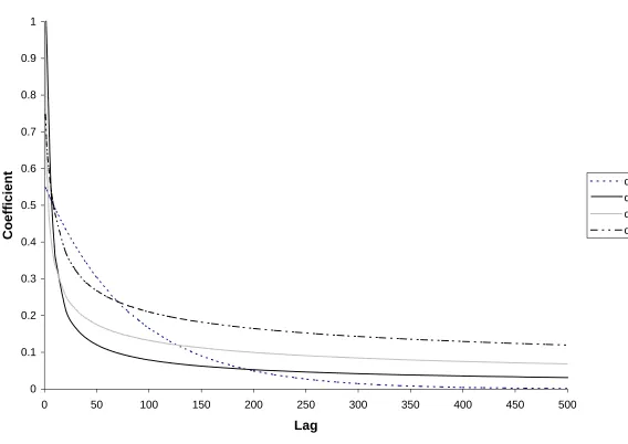
The estimates obtained here for φ and ψ , namely -0.27 and 0.68 for the most

general specification, are rather different to the 0.78 and -0.68 given by Bollerslev and

Mikkelsen (1999, Table 1), although the estimates of d are similar, namely 0.59 and

0.65. However, the moving-average representations obtained from these sets of

parameters estimates are qualitatively similar. This is shown on Figure 1 that compares

the moving-average coefficients ψ _j defined by equation (21). The coefficients are

positive and monotonic decreasing for the four sets of parameter values used to produce

Figure 1. They show the expected hyperbolic decay when d >0 and a geometric decay

when d =0. The values of b_j in equations (19) and (24) that are used to calculate the

conditional variances decay much faster. For each of the four curves shown on Figure

The results reported in Table 1 are for a constant conditional mean, µ_t =µ.

Alternative specifications such as µ_t =µ +βr_t−1, _t h_t

2 1

− =µ

µ and µ_t =µ +λ h_t

give similar values of the log-likelihood when the volatility parameters are set to the

values in the final row of Table 1. First, including the lagged return r_t−1 is not

necessary because the first-lag autocorrelation of the S&P 100 returns equals -0.022

and is statistically insignificant. Second, including the adjustment −₂1h_t makes the

conditional expectation of

1 1

− −

−

t t t

p p p

constant when the conditional distribution is

Normal. The adjustment reduces the log-likelihood by an unimportant 0.3. Third,

incorporating the ARCH-M parameter λ gives an optimal value of 0.10 and an

increase in the log-likelihood of 1.5. This increase is not significant using a non-robust

likelihood-ratio test at the 5% level.

3.3. Stochastic volatility specifications

Two shocks per unit time characterise stochastic volatility (SV) models, in contrast to

the single shock z_t that appears in ARCH models. A general framework for long

memory stochastic volatility models is given for returns r_t by

t t

t u

r =µ+σ (25)

with ln

( )

( )

(

) (

) (

)

This framework has been investigated by Breidt, Crato and de Lima (1998), Harvey

(1998) and Bollerslev and Wright (2000), all of whom provide results for the

simplifying assumption that the two i.i.d. processes

{ }

{ }

assumption can be relaxed and has been for short memory applications (Taylor, 1994,

Shephard, 1996).

Parameter estimation is difficult for SV models, compared with ARCH models,

because SV models have twice as many random innovations as observable variables.

Breidt, Crato and de Lima (1998) describe a spectral-likelihood estimator and provide

results for a CRSP index from 1962 to 1989. For the ARFIMA(1, d, 0) specification

they estimate d =0.44 and φ =0.93. Bollerslev and Wright (2000) provide detailed

simulation evidence about semiparametric estimates of d, related to the frequency of

the observations.

It is apparent that the ARCH specification (15)-(17) has a similar structure to

the SV specification (25)-(26). Short memory special cases of these specifications,

given by d =q=0, have similar moments (Taylor, 1994). This is a consequence of the

special cases having the same bivariate diffusion limit when appropriate parameter

values are defined for increasingly frequent observations (Nelson, 1990, Duan, 1997).

It seems reasonable to conjecture that the multivariate distributions for returns defined

by (15)-(17) and (25)-(26) are similar, with the special case of independent shocks

{ }

4. Option pricing methodology

4.1. A review of SV and ARCH methods

The pricing of options when volatility is stochastic and has a short memory has been

studied by several researchers using a variety of methods. The most popular methods

commence with separate diffusion specifications for the asset price and its volatility.

These are called stochastic volatility (SV) methods. Option prices then depend on

several parameters including a volatility risk premium and the correlation between the

differentials of the Wiener processes in the separate diffusions. Hull and White (1987)

provide solutions that include a simple formula when volatility risk is not priced and

the correlation between the differentials is zero. The closed form solution of Heston

(1993) assumes that volatility follows a square-root process and permits a general

correlation and a non-zero volatility risk premium; for applications see, for example,

Bakshi, Cao and Chen (1997, 2000) and for extensions see Duffie, Pan and Singleton

(2000).

There is much less research into option pricing for short memory ARCH

models. Duan (1995) provides a valuation framework and explicit results for the

GARCH(1,1) process that can be extended to other ARCH specifications. Ritchken and

Trevor (1999) provide an efficient lattice algorithm for GARCH(1,1) processes and

extensions for which the conditional variance depends on the previous value and the

Methods for pricing options when volatility has a long memory have been

described by Comte and Renault (1998) and Bollerslev and Mikkelsen (1996, 1999).

The former authors provide analysis within a bivariate diffusion framework. They

replace the usual Wiener process in the volatility equation by fractional Brownian

motion. However, their option pricing formula appears to require independence

between the Wiener process in the price equation and the volatility process. This

assumption is not consistent with the empirical evidence for stock returns. The

assumption is refuted, for example, by finding that θ is not zero in the function g

( )

that appears in an exponential ARCH model.

The most practical way to price options with long memory in volatility is

probably based upon ARCH models, as demonstrated by Bollerslev and Mikkelsen

(1999). We follow the same strategy. From the asymptotic results in Duan (1997), also

discussed in Ritchken and Trevor (1999), it is anticipated that insights about options

priced from a long memory ARCH model will be similar to the insights that can be

obtained from a related long memory SV model.

4.2. The ARCH pricing framework

When pricing options it will be assumed that returns are calculated from prices (or

index levels) as r_t =ln

(

)

interest rate and a constant dividend yield will also be assumed and, to simplify the

per trading period. Conditional expectations are defined with respect to current and

prior price information represented by I_t =

{

}

To obtain fair option prices in an ARCH framework it is necessary to make

additional assumptions in order to obtain a risk-neutral measure Q. Duan (1995) and

Bollerslev and Mikkelsen (1999) provide sufficient conditions to apply a risk-neutral

valuation methodology. For example, it is sufficient that a representative agent has

constant relative risk aversion and that returns and aggregate growth rates in

consumption have conditional normal distributions. Kallsen and Taqqu (1998) derive

the same solution as Duan (1995) without making assumptions about utility functions

and consumption. Instead, they assume that intraday prices are determined by

geometric Brownian motion with volatility determined once a day from a discrete-time

ARCH model.

At time t', measured in trading periods, the fair price of an European contingent

claim that has value y_t'+n

(

)

(

)

[ _{' ' '}

' t n t n t

n Q

t E e y p I

y = −ρ _{+ +} (27)

with ρ the risk-free interest rate for one trading period. Our objective is now to specify

an appropriate way to simulate p_t'+n under a risk-neutral measure Q and thereby to

evaluate the above conditional expectation using Monte Carlo methods.

Following Duan (1995), it is assumed that observed returns are obtained under a

probability measure P from

(

)

1 P t t t

t I N h

r ₋ µ (28)

( )

= (29)

and that in a risk-neutral framework returns are obtained under measure Q from

(

)

~

2 1

1 t t

Q t

t I N h h

r ₋ ρ−δ − (30)

with

(

)

_{( )}

= ρ δ . (31)

Here δ is the dividend yield, that corresponds to a dividend payment of d_t =

( )

per share at time t. Then EQ

[

]

one share and the dividend payment is EQ

[

]

risk-neutral framework.

Note that the conditional means are different for measures P and Q but the

functions h_t

(

)

are identical. Duan (1995) proves that this is a consequence of the sufficient

assumptions that he states about risk preferences and distributions. The same

conclusion applies for the less restrictive assumptions of Kallsen and Taqqu (1998).

Option prices depend on the specifications for µ_t and h_t. We again follow

Duan (1995) and assume that

t t

t ρ δ h λ h

µ = − −₂1 + ₍₃₂₎

with λ representing a risk-premium parameter. Then the conditional expectations of r_t

.

* _=−λ

− _t

t z

z (33)

4.3. Long memory ARCH equations

Option prices are evaluated in this paper when the conditional variances are given by

the ARMA(N, 1) approximation to the FIEGARCH(1, d, 1) specification. From (17),

(24) and (33),

( )

(

) (

) ( ) (

)

(

)

1 ₁ *₁

1

λ ψ

ψ

α = + = + −

−     ∑ − _{− −}

= t t t

N

j j

jL h L g z L g z

b (34)

and

( )

(

)

g _t =θ _t +γ _t − (35)

with the autoregressive coefficients b_j defined by (19) as functions of φ and d; also

π / 2

=

C for conditional normal distributions2. Suppose there are returns observed at

times 1≤t≤t', whose distributions are given by measure P, and that we then want to

simulate returns for times t>t' using measure Q. Then ln

( )

1 '

1≤t ≤t+ using the observed returns, with ln

( )

( )

followed by simulating z_t* ~Q N(0,1) and hence obtaining r_t and ln

( )

2

When z~ N(0,1),

[

]

( )

(

( )

)

2

1 + Φ −

− =

−λ π λ λ λ

z

E with Φ the cumulative

The expectation of ln

( )

measure P. It is different for measure Q because

(

)

[

]

(

[ ]

)

2 / 2 2 * *_{− =− + − − ≅− +} t Q t Q z E z g

E (36)

when λis small, and this expectation is in general not zero. For a fixed t', as t →∞,

( )

[

]

(

)

[

(

)

]

    ∑ − + → − = * 1 1

' 1 1

ln N Q _t

j j t t Q z g E b I h

E . (37)

The difference between the P and Q expectations of ln

( )

volatility risk premium. This "premium" is typically negative, because typically

0 ,

0 ≤

> θ

λ and γ >0. Furthermore, when θ is negative the major term in (36) is

λθ

− , because λ is always small, and then the "premium" reflects the degree of

asymmetry in the volatility shocks g

( )

The magnitude of the volatility "risk premium" can be important and, indeed,

the quantity defined by the limit in (37) becomes infinite4 as N →∞ when d is

positive. A realistic value of λ for the S & P 100 index is 0.028, obtained by assuming

that the equity risk premium is 6% per annum5. For the short memory parameter values

in the first row of Table 1, when d =0 and N =1000, the limit of EQ

[

( )

]

3

The dependence of moments of h_t on the measure is shown by Duan (1995, p. 19) for

the GARCH(1,1) model.

4

As

(

)

1 1 ∑ = ∑ =∞ = ∞

= j j

j j

b a

5

The conditional expectations of r_t for measures P and Q differ by λ h_t and a typical

average value of h_t is 0.00858. Assuming 253 trading days in one year gives the

equals 0.10. This limit increases to 0.20 for the parameter values in the final row of

Table 1, when d =0.4 and N =1000. The typical effect of adding 0.2 to ln

( )

multiply standard deviations h_t by 1.1 so that far-horizon expected volatilities, under

Q, are slightly higher than might be expected from historical standard deviations.

Consequently, on average the term structure of implied volatilities will slope upwards.

4.4. Numerical methods

The preceding equations can be used to value an European contingent claim at time t'

by simulating prices under the risk-neutral measure Q, followed by estimating the

expected discounted terminal payoff at time t'+n as stated in equation (27). Two

variations on these equations are used when obtaining representative results in Section

5. First, the specification of µ_t can be different for times on either side of t' to allow

for changes through time in risk-free interest rates and risk premia. Equation (32) is

then replaced by

'. , , ' , ' 2 1 2 1 t t h h t t h h m t t t t t > + − − = ≤ + − = λ δ ρ λ µ (38)

Second, because the observed conditional distributions are not Normal whilst the

simulations assume that they are, it is necessary to define

'. , 2 , ' , ' t t t t C C > = ≤ =

for a constant C' estimated from observed returns. An alternative method, described by

Bollerslev and Mikkelsen (1999), is to simulate from the sample distribution of

standardised observed returns.

Standard variance reduction techniques can be applied to increase the accuracy

of Monte Carlo estimates of contingent claim prices. A suggested antithetic method

uses one i.i.d. N(0,1) sequence

{ }

{ }

t

z

− ,

{ }

{ }

between z_t* and z_t• ; this is achieved by defining Φ

( ) ( )

( )

four sequences provide claim prices whose average, y say, is much less variable than

the claim price from a single sequence. An overall average yˆ is then obtained from a

set of K values

{

}

The control variate method makes use of an unbiased estimate yˆ_CV of a known

parameter y_CV , such that yˆ is positively correlated with yˆ_CV . A suitable parameter,

when pricing a call option in an ARCH framework, is the price of a call option when

volatility is deterministic. The deterministic volatility process is defined by replacing

all terms ln

( )

Then y_CV is given by a simple modification of the Black-Scholes formula, whilst yˆ_CV

is obtained by using the same 4K sequences of i.i.d. variables that define yˆ. Finally, a

more accurate estimate of the option price is then given by ~y = yˆ−β

(

)

5. Illustrative long memory option prices

5.1. Inputs

The Black-Scholes formula has six parameters, when an asset pays dividends at a

constant rate, namely the current asset price S, the time until the exercise decision T, the

exercise price X, the risk-free rate R, the dividend yield D and the volatility σ. There

are many more parameters and additional inputs for the FIEGARCH option pricing

methodology described in Section 4. To apply that methodology to value European

options it is necessary to specify eighteen numbers, a price history and a random

number generator, as follows :

• Contractual parameters - time until exercise T measured in years, the exercise price

X and whether a call or a put option.

• The current asset price S = p_t' and a set of previous prices

{

}

• Trading periods per annum M, such that consecutive observed prices are separated

by 1/M years and likewise for simulated prices

{

}

• Risk-free annual interest rate R, from which the trading period rate ρ =R/M is

obtained.

• Annual dividend yield D giving a constant trading period payout rate of

M D/ =

δ ; both R and D are continuously compounded and applicable for the life

• The risk premium λ for investment in the asset during the life of the option, such

that one-period conditional expected returns are µ_t = ρ−δ −₂1h_t +λ h_t .

• Parameters m and λ' that define conditional expected returns during the time period

of the observed prices by µ_t =m−₂1h_t +λ' h_t .

• Eight parameters that define the one-period conditional variances h_t. The

integration level d, the autoregressive parameter φ and the truncation level N

determine the parameters b_j (given by equation (19)) of the AR(N) filter in

equation (34). The mean α and the moving-average parameter ψ complete the

ARMA(N, 1) specification for ln

( )

the ARMA(N, 1) process depend on γ and θ, that respectively appear in the

symmetric function γ

(

)

determines the shock term g

( )

prices but equals 2π when returns are simulated.

• K, the number of independent simulations of the terminal asset price S_T = p_t'+n.

• A set of Kn pseudo-random numbers distributed uniformly between 0 and 1, from

which pseudo-random standard normal variates can be obtained. These numbers

typically depend on a seed value and a deterministic algorithm.

Option values are tabulated for hypothetical European options on the S & P 100 index.

Options are valued for ten dates defined by the last trading days of the ten years from

1989 to 1998 inclusive. For valuation dates from 1992 onwards the size of the price

history is set at t'=2000; for previous years the price history commences on 6 March

1984 and t'<2000. It is assumed that there are M =252 trading days in one year and

hence exactly 21 trading days in one simulated month. Option values are tabulated

when T is 1, 2, 3, 6, 12, 18 and 24 months.

Table 2 lists the parameter values used to obtain the main results. The

annualised risk-free rate and dividend yield are set at 5% and 2% respectively. The risk

parameter λ is set at 0.028 to give an annual equity risk premium of 6% (see footnote

5). The mean return parameter m is set to the historic mean of the complete set of S & P

100 returns from March 1984 to December 1998 and λ' is set to zero.

There are two sets of values for the conditional variance process because the

primary objective here is to compare option values when volatility is assumed to have

either a short or a long memory. The long memory parameter set takes the integration

level to be d =0.4 because this is an appropriate level based upon the recent evidence

from high-frequency data, reviewed in Section 2.3. The remaining variance parameters

are then based on Table 1; as the moving-average parameter is small it is set to zero and

filter6 is truncated at lag 1000, although the results obtained will nevertheless be

referred to as long memory results. The short memory parameters are similar to those

for the AR(1) estimates provided in Table 1. The parameters γ and θ are both 6% less

in Table 2 than in Table 1 to ensure that selected moments are matched for the short

and long memory specifications; the unconditional mean and variance7 of ln

( )

then matched for the historic measure P, although the unconditional means differ by

approximately 0.10 for the risk-neutral measure Q as noted in Section 4.3.

Option prices are estimated from K =10,000 independent simulations of prices

{

}

described in Section 4.4 then produces results for a long memory process in about 50

minutes, using a PC running at 466 MHz. Most of the time is spent evaluating the

high-order AR filter; the computation time is less than 5 minutes for the short memory

6

This filter is

(

)(

)

(

)

Also, b₆ >b_j >b_j+1>0 for j >6, b₁₀₀ =0.00017, b₁₀₀₀ =7×10−6

and ∑

=

1000

1

j j

b equals 0.983.

7

I thank Granville Tunnicliffe-Wilson for calculating the variance of the AR(1000)

process. Separate seed values are used to commence the "random number" calculations8

for the ten valuation dates; these seed values are always the same for calculations that

have the same valuation date.

5.3. Comparisons of implied volatility term structures

The values of all options are reported using annualised implied volatilities rather than

prices. Each implied volatility (IV) is calculated from the Black-Scholes formula,

adjusted for continuous dividends. The complete set of IV outputs for one set of inputs

forms a matrix with rows labelled by the exercise prices X and columns labelled by the

times to expiry T; examples are given in Tables 5 and 6 and are discussed later.

Initially we only consider at-the-money options, for which the exercise price

equals the forward price F =Se(R−D)T, with IV values obtained by linear interpolation

across two adjacent values of X. As T varies, the IV values represent the term structure

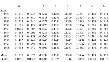
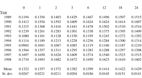
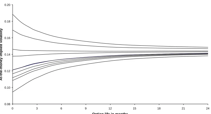
of implied volatility. Tables 3 and 4 respectively summarise these term structures for

the short and long memory specifications. The same information is plotted on Figures 2

and 3 respectively. The IV values for T =0 are obtained from the conditional variances

on the valuation dates. The standard errors of the tabulated implied volatilities increase

with T. The maximum standard errors for at-the-money options are respectively 0.0003

and 0.0004 for the short and long memory specifications.

8

The Excel VBA pseudo-random number generator was used. This generator has cycle

length 224. Use is made of 30% of the complete cycle when K =10,000 and

504 =

The ten IV term structures for the short memory specification commence

between 9.5% (1993) and 18.8% (1997) and converge towards the limiting value of

14.3%. The initial IV values are near the median level from 1989 to 1991, are low from

1992 to 1995 and are high from 1996 to 1998. Six of the term structures slope upwards,

two are almost flat and two slope downwards. The shapes of these term structures are

completely determined by the initial IV values because the volatility process is

Markovian.

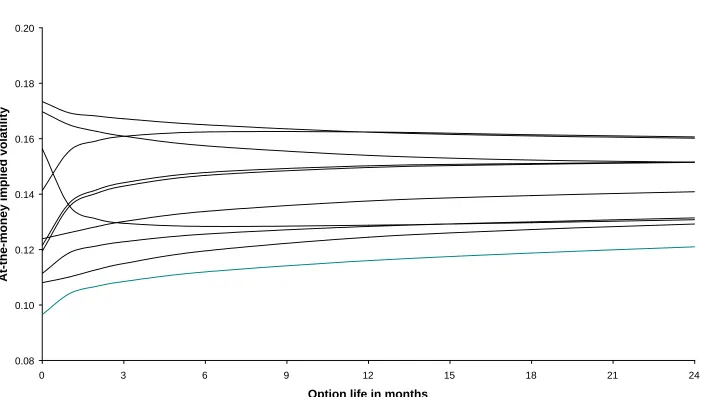
There are three clear differences between the term structures for the short and

long memory specifications that can be seen by comparing Figures 2 and 3. First, the

long memory term structures can and do intersect because the volatility process is not

Markovian. Second, some of the term structures have sharp kinks for the first month.

This is particularly noteworthy for 1990 and 1996 when the term structures are not

monotonic. For 1990, the initial value of 14.1% is followed by 15.6% at one month and

a gradual rise to 16.2% at six months and a subsequent slow decline. For 1996, the term

structure commences at 15.6%, falls to 13.6% after one month and reaches a minimum

of 12.8% after six months followed by a slow incline. The eight other term structures

are monotonic and only those for 1997 and 1998 slope downwards. Third, the term

structures approach their limiting value very slowly9. The two-year IVs range from

12.1% to 16.1% and it is not possible to deduce the limiting value, although 15.0% to

9

The results support the conjecture that IV(T)≅a₁+a₂T2d−1 for large T with a₂

16.0% is a plausible range10. It is notable that the dispersion between the ten IV values

for each T decreases slowly as T increases, from 2.2% for one-month options to 1.4%

for two-year options.

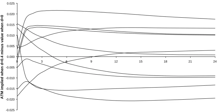
There are substantial differences between the two IV values that are calculated

for each valuation date and each option lifetime. Figure 4 shows the differences

between the at-the-money IVs for the long memory specification minus the number for

the short memory specification. When T =0 these differences range from -1.9%

(1997) to 1.5% (1992), for three-month options from -1.5% (1995, 1996) to 2.1%

(1990) and for two-year options from -1.9% (1995) to 1.7% (1990). The standard

deviation of the ten differences is between 1.1% and 1.4% for all values of T

considered so it is common for the short and long memory option prices to have IVs

that differ by more than 1%.

5.4. Comparisons of smile effects

The columns of the IV matrix provide information about the strength of the so-called

smile effect for options prices. These effects seem to be remarkably robust to the choice

of valuation date and they are not very sensitive to the choice between the short and

10

An estimate of the constant a₁ (defined in the previous footnote) is 16.0%. An

estimate of 15.0% follows by supposing the long memory limit is 105% of the short

memory limit, based on the limit of ln

( )

process as noted in Section 4.3. The difference in the limits is a consequence of the risk

premium obtained by owning the asset; its magnitude is mainly determined by the

long memory specifications. This can be seen by considering the ten values of

) , ( ) ,

(T X₁ IV T X₂

IV

IV = −

∆ obtained for the ten valuation dates, for various values

of T, various pairs of exercise prices X₁,X₂ and a choice of volatility process. First,

for one-month options with S =100, X₁=92 and X₂ =108, the values of ∆IV range

from 3.0% to 3.3% for the short memory specification and from 3.7% to 4.0% for the

long memory specification. Second, for two-year options with X₁ =80 and X₂ =120,

the values of ∆IV range from 1.8% to 2.0% and from 1.8% to 1.9%, respectively for

the short and long memory specifications.

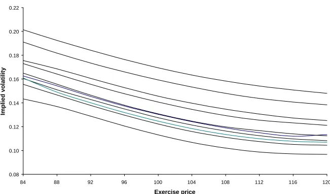
Figure 5 shows the smiles for three-month options valued using the short

memory model, separately for the ten valuation dates. As may be expected from the

above remarks the ten curves are approximately parallel to each other. They are almost

all monotonic decreasing for the range of exercise prices considered, so that a U-shaped

function (from which the idea of a smile is derived) can not be seen. The near

monotonic decline is a standard theoretical result when volatility shocks are negatively

correlated with price shocks (Hull, 2000). It is also a stylized empirical fact for U.S.

equity index options, see, for example, Rubinstein (1994) and Dumas, Fleming and

Whaley (1998).

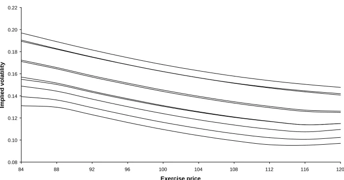
Figure 6 shows the three-month smiles for the long memory specification. The

shapes on Figures 5 and 6 are similar, as all the curves are for the same expiry time, but

they are more dispersed on Figure 6 because the long memory effect induces more

dispersion in at-the-money IVs. The minima of the smiles are generally near an

when the forward price is 106.2. The parallel shapes are clear; the two highest curves

are almost identical, and the third, fourth and fifth highest curves are almost the same.

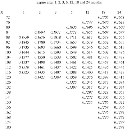
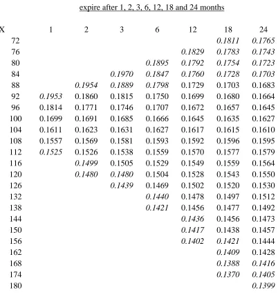
Tables 5 and 6 provide matrices of implied volatilities for options valued on 31

December 1998. When either the call or the put option is deep out-of-the-money it is

difficult to estimate the option price accurately because the risk-neutral probability

) (X

q of the out-of-the-money option expiring in-the-money is small. Consequently, the

IV information has not been presented when the corresponding standard errors exceed

0.2%; estimates of q(X) are less than 3%. The standard errors of the IVs are least for

options that are near to at-the-money and most of them are less than 0.05% for the IVs

listed in Tables 5 and 6. All the sections of the smiles summarised by Tables 5 and 6

are monotonic decreasing functions of the exercise price. The IV decreases by

approximately 4% to 5% for each tabulated section.

5.5. Sensitivity analysis

The sensitivity of the IV matrices to three of the inputs has been assessed for options

valued on 31 December 1998. First, consider a change to the risk parameter λ that

corresponds to an annual risk premium of 6% for the tabulated results. From Section

4.3, option prices should be lower for large T when λ is reduced to zero. Changing λ

to zero reduces the at-the-money IV for two-year options from 16.0% to 15.4% for the

long memory inputs, with a similar reduction for the short memory inputs. Second,

consider reducing the truncation level N in the AR(N) filter from 1000 to 100. Although

the IV numbers by appreciable amounts and can not be recommended; for example, the

two-year at-the-money IV then changes from 16.0% to 14.7%.

The smile shapes on Figures 5, 6 and 7 are heavily influenced by the negative

asymmetric shock parameter θ, that is substantial relative to the symmetric shock

parameter γ . The asymmetry in the smile shapes can be expected to disappear when θ

is zero, which is realistic for some assets including exchange rates. Figures 8 and 9

compare smile shapes when θ is changed from the values used previously to zero, with

γ scaled to ensure the variance of ln

( )

that the one-month smile shapes become U-shaped when θ is zero, whilst Figure 9

shows that the IV are then almost constant for one-year options.

6.

Conclusions

The empirical evidence for long memory in volatility is strong, for both equity

(Andersen, Bollerslev, Diebold and Ebens, 2000, Areal and Taylor, 2000) and foreign

exchange markets (Andersen, Bollerslev, Diebold and Labys, 2000). This evidence may

more precisely be interpreted as evidence for long memory effects, because there are

short memory processes that have similar autocorrelations and spectral densities, except

at very low frequencies (Gallant, Hsu and Tauchen, 1999, Barndorff-Nielsen and

Shephard, 2001). There is also evidence that people trade at option prices that are more

compatible with a long memory process for volatility than with a parsimonious short