Munich Personal RePEc Archive
Estimating Term Structure Changes
using Principal Component Analysis in
Indian Sovereign Bond Market
Nath, Golaka
4 June 2012
Online at
https://mpra.ub.uni-muenchen.de/39229/
[email protected] 1
Estimating Term Structure Changes using Principal Component Analysis in Indian Sovereign Bond Market
Golaka C Nath
This paper analyses the India sovereign yield to find out the principal factors affecting the term structure of
interest rate changes. We apply Principal Component Analysis (PCA) on our data consisting of zero coupon interest
rates derived from government bond trading using Nelson-Siegel functional form. This decomposition of the yield
curve highlights important relationship between identified factors and metrics of the term structure shape. The
empirical findings support statistical similarities between the Indian yield curve and term structure studies of
major countries.
Key words: Indian Sovereign Yield Curve, principal component, interest rates, bond, yield curve, macroeconomics, term structure of interest rates
[email protected] 2
1. Introduction
Yield curve estimation in emerging markets like India has been a challenging job. The sovereign bond market is
characterized by illiquidity in terms of number of bonds traded vis-à-vis number of outstanding bonds, value
traded as a proportion to outstanding bond issuances, activity concentrated on few bonds and the benchmark
10-year bond typically account for a large share in trading activity, low trading activity in major part of the yield curve.
Hence estimation of the sovereign yield curves have to be done using sophisticated methods. Entities like National
Stock Exchange (NSE) and Clearing Corporation of India Ltd (CCIL) have been doing a fair job by estimating the term
structure on daily basis and releasing the same to the market. Before CCIL came to the arena and specifically after
the introduction of anonymous order matching system in Gilts market in August 2005, NSE captured the trading
data of the sovereign bond market through their Wholesale Debt Market (WDM) platform as major part of the
deals in the market used to be transacted through brokers. It could not capture all deals in the market as some of
the deals were transacted directly among market participants and settlement of all trades happened at Reserve
Bank of India (RBI). It helped NSE to estimate the term structure on daily basis using Nelson-Siegel functional form
and many banks and institutions adopted the valuation techniques using the information of the estimated term
structure. The role of CCIL became very important after Reserve Bank of India mandated settlement of all
Government securities deals through CCIL. Since all trades, including the brokered trades, have to be reported to a
centralized system at RBI for final settlement through CCIL, it became the repository of all trades in Gilts in India.
Unlike NSE, this helped CCIL in capturing the full market data in Gilts and since it has to provide guarantee of
settlement, it estimated the term structure of interest rates on daily basis using Nelson-Siegel functional form.
Indian sovereign bond market is generally illiquid when we compare it to the developed markets. However, the
well-functioning market microstructure helped it to have a great deal of market efficiency in pricing instruments
traded in the market. The well-structured primary issuances market for Government bonds through Issuance
calendars, availability of bonds in all maturities upto 30 years, higher level of outstanding issuances in many bonds
of different maturities, passive consolidation of issuances through reopening issues and creating liquidity, a
well-functioning primary dealers network, a central counterparty (CCP) based settlement system, availability of quality
information to market participants on each and every bond through CCIL, creating an anonymous order drive
system for sovereign bonds, a well-functioning money market for short term market using three different variants
like Inter-bank call, inter-bank Repo and a quasi-repo CBLO (Collateralized Borrowing and Lending Obligations), a
well-designed Liquidity Adjustment Facility (LAF) of RBI to support the market to moderate the money supply using
daily fixed rate Repo and Reverse Repo, etc. has helped the market in terms of price efficiency.
A reasonable estimation of the sovereign yield curve in an economy is important for several reasons, both at the
[email protected] 3
economy as private corporate entities raise funds by paying a credit spread for the risk inherent in them; investors
use the sovereign yield curves to demand an appropriate price for their investment risk; banks and other financial
institutions use the yield curves to not only price the illiquid securities in their books but also match the duration of
their assets and liabilities; central banks use the information from secondary market yield curves to monitor the
policy interest rate synchronization with the “economic effective rate” in the inter-bank market; at macroeconomic level, the yield curve has a predictive power for the state of economy. The yield curve modeling
has become an important area for all financial markets. During the last few years, we could observe high volatility
of interest rates. The yield of corporate and government bonds have increased significantly during the financial
crisis. Due to current debt crisis on the periphery of European monetary union, bond yields remain at high level. In
India, yields have remain high for a long period as the inflation has remained high for good many months and
liquidity shortage in the inter-bank market has been continuing unabated since July 2010.
Term structure estimation using models like Nelson-Siegel (NS) functional form has been in operation in India since
1999. The parameters estimated by this model helps us to calculate the spot interest rate (zero rate) for any term
using the NS equation. The risk management practices like Value-at-Risk (VaR) heavily depend on the historical
price behavior to estimate the possible future risk for having the sufficient amount of capital to cover market risk
in those investments; it is paramount to simulate the historical price of the securities using the historical yield
curves. The market observed price of the bonds cannot be used to compute VaR as a bond changes its structure
every day (maturity comes down by 1 day on daily basis and hence a 10-year bond today was a 11-year bond one
year back and hence its observed trading prices were on the basis of time to maturity and other factors). The
purpose of this study is to understand the dynamics of the term structure of interest rate in India using Principal
Component Analysis (PCA). The main purpose of this paper is to study the term structure dynamics and to figure
out the common factors of the Indian term structure and its volatility as it helps to understand the pricing
mechanism of various OTC and other underlying and derivative products. Corporate entities price their issuances
on the basis of sovereign yield by adding a credit spread. Previous literature has focused on the term structure of
interest rates (Litterman and Scheinkman, 1991; Dai and Singleton, 2000). These studies have concluded that a few
common factors explain observed variation in historical bond prices. These three common factors in the term
structure of interest rates are interpreted as level, slope and curvature factors based on the factor loadings from
principal components analysis (Díaz et al., 2010b). This principal component analysis is a common method to
analyse the bond valuation ability of alternative models on the first moment of interest rates (Litterman and
Scheinkman, 1991; Piazzesi, 2005; Matzner-Løber and Villa, 2004; Pérignon et al., 2007; Cornillon et al., 2008;
Olawale and Garwe, 2010; and Huang and Chen, 2011). Chandra (2008) studied Indian yield curve movements
[email protected] 4
The paper is divided into different sections: Section 2 provides the dynamics of historical term structure of interest
rates; Section 3 provides the volatility of the term structure; Section 4 gives the use of PCA in studying dynamics of
yield curve; Section 5 estimates the dynamics of term structure using PCA, Section 6 gives the conclusion and
findings of the study.
2. Historical Term Structure of Interest Rate in India
Study of yield curve behavior has been an import part of financial market research as it provides us important
information about the future expectation of growth, inflation, recession, etc. The slope change of the yield curves
provides good information about the future of the economy (Estrella & Mishkin, 1996; Bernanke & Blinder, 1992;
Mishkin, 1990). Indian sovereign bond market has seen many structural changes during last two decades or so.
Many significant microstructure changes were introduced during last few years to strengthen Indian sovereign
bond market. The issuance of sovereign bonds has become increasingly systematic with passive consolidation.
Very few issues were new issues and RBI concentrated in reopening the issues to add liquidity as outstanding
stocks increased due to re-issuances. The borrowing of the Government considerably increased over time to fund a
growing economy and reached `30.5trillion as of March’12 (Table - 1).
Table – 1: Government Securities Issuance
Year Change over Previous Year (%) Debt (`Trillion)
Average Coupon (%)
Average Maturity (years)
Turnover Ratio
2006-07 19.05 12.97 8.66 10.1 78.76 2007-08 21.06 15.70 9.57 8.42 105.33 2008-09 18.22 18.56 8.22 9.91 116.37 2009-10 16.95 21.71 7.98 9.79 134.22 2010-11 14.76 24.91 7.84 9.76 115.24 2011-12 22.43 30.50 7.87 9.69 114.37 Note: Borrowing included dated securities, floating rate bonds, T-bills issued by Govt. of India and Turnover Ratio has been calculated as the ratio of 12 months total trading value and total outstanding debt.
The primary issuances of Government securities are managed by RBI as per a statute. The RBI also works as the
central depository and record keeper of the Government debt. For historical reasons, the Government securities
market was a typical Over the Counter (OTC) market where banks and financial institutions traded among
themselves and settled at central bank money. A large financial market scam in 1992 involving Government
securities, brokers and Banks resulted in making the securities holding records into electronic book entry form
from the physical from. The clear differentiation between constituent and proprietary positions and holding
helped creating audit trail which helped the market in many ways in terms of transparency. The WDM segment of
NSE started in June’94 and it revolutionized the transparency system in Government securities market. NSE made
it mandatory for brokers to report the deals to its electronic platform as most of the deals in Gilts were broker
driven. Once the deals were reported to the platform, NSE initiated the dissemination of the same to the market
[image:5.612.76.533.345.478.2][email protected] 5
data. NSE started using the deals to estimate yield curves and made the Zero coupon yield curves public from
1999.
The RBI introduced an electronic reporting system in Feb’02 making it mandatory for market participants (as most
buyers and sellers are Banks and financial institutions) to report the deals within a limited time to its reporting
system called Negotiated Dealing system (NDS). Once the deals were reported to the system, it could be
consolidated fro settlement using a Delivery versus Payment – II mechanism through CCIL which worked as a
clearing house and a CCP. As a part of reforming financial market structure in India, RBI made it mandatory for all
Banks and financial institutions to settle their deals in Government securities (outright and Repo) through CCIL
from Feb’02. To add to transparency, RBI also introduced an anonymous order matching system sans brokers for Government securities in Aug’05. This resulted in a dramatic change in the market microstructure. Brokers became increasingly redundant as market participants started trading using the anonymous order matching system and
within a very short span of time, about 80% of the market deals became deals without the convenience of the
brokers. As all deals were being settled through CCIL, it started disseminating important information about the
market to improve transparency in the market. CCIL also started estimating Zero curves and used the same for
valuation and margining purpose. CCIL also introduced Delivery versus Payment –II mechanism in April’04 and
added further comfort to the market.
Interest rate cycle in India moved from high interest regime to low interest rate regime and back to high interest
regime during period under our study. There have been some important regulatory changes through introduction
of Primary Dealers system and structured auction system using multiple pricing mechanisms. The Fiscal
Responsibility and Budget Management Act (FRBM) helped RBI to move away from supporting primary auctions as
devolvement of debt was shifted to Primary Dealers as they became underwriters of the Government securities
issuances. The trading activity showed significant changes during the financial years from 2003-04 and 2011-12. It
declined during three financial years while increased during other years for which we have used the data (Table -2)
for our study.
Table – 2: Trading Activity in Government Securities Market
Financial Years (Apr – Mar) Change in Market Activity (%)
2003-04 46.37
2004-05 -27.99
2005-06 -23.76
2006-07 18.13
2007-08 61.90
2008-09 30.62
2009-10 34.89
2010-11 -1.47
2011-12 21.50
[email protected] 6
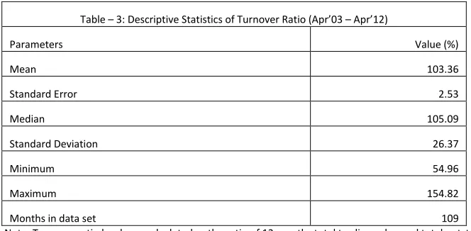
However, the Indian Government bond market remained relatively illiquid and the turnover ratio during April’03
and April’12 varied between 55% and 155% (Table -3). The market heavily depended on domestic institutions for its growth as investment from Foreign Institutional Investors (FII) was restricted with administrative caps. Trading
was restricted to few securities and high concentration was on the 5 and 10 year benchmark securities though
Government has been issuing securities upto 30 years of maturity.
Table – 3: Descriptive Statistics of Turnover Ratio (Apr’03 –Apr’12)
Parameters Value (%)
Mean 103.36
Standard Error 2.53
Median 105.09
Standard Deviation 26.37
Minimum 54.96
Maximum 154.82
Months in data set 109
Note: Turnover ratio has been calculated as the ratio of 12 months total trading value and total outstanding debt.
NSE and CCIL have been using Nelson-Siegel functional form for estimation of spot yield curves. Nelson-Siegel
functional form is a straight forward equation to estimate the yield of a particular term/tenor/maturity suing the
estimated 4 parameters. The simplistic N-S equation can be solved by an iterative method as it has 4 unknowns in
one equation.
( )
(
) (
( ))
( )We used the parameters β0, β1, β2 and τ to estimate the appropriate rates for any term, m. We selected maturities,
m’s, ranging from 3-month to 30 years at appropriate terms like 3-month, 6-month, 1-year, 2-year, 5-year, 7-year, 10-year, 12-year, 15-year, 20-year, 25-year and 30-year and calculated the time series of yields of these maturities
from 01-April-1999 to 12-May-2012. For smoothing purpose, we converted the daily interest rate data into
monthly data series by taking monthly averages. This resulted in about 158 monthly observations. We estimated
[image:7.612.141.473.181.344.2][email protected] 7
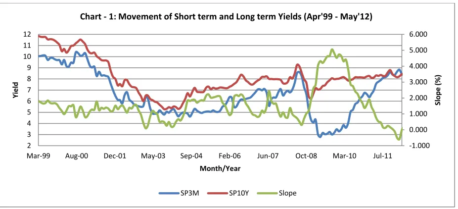
We analysed the descriptive statistics (Table - 3) of the yields and found that the difference between maximum
and minimum yield are far higher in the short term than the long term. This is due to the fact that the short term
rates are more guided by monetary policy rates and liquidity factors. In the aftermath of financial crisis in 2007-08,
RBI supported the market by infusing huge liquidity along with bringing down policy Repo rate and reserve ratios
for the Banks. This helped in lower interest rates at the shorter end but the longer end remained more stable. The
liquidity premia was highest for the 5 year security followed by 10 year and seven years. This replicates the market
structure as large number of deals happens in the market within 5 to 10 year maturities.
Table – 3: Descriptive Statistics of Historical term Structure of Interest Rate (%) 3
Months
6
Months 1 Year 2 year 5 year 7 Year 10 year 12 year 15 year 20 year 25 year 30 year Mean 6.5735 6.6356 6.7606 6.9990 7.5637 7.8284 8.1154 8.2572 8.4215 8.6126 8.7425 8.8363 Std Dev 1.9365 1.8490 1.7249 1.5998 1.5482 1.5730 1.6072 1.6219 1.6341 1.6404 1.6399 1.6380 Max 10.4018 10.3837 10.3807 10.5276 11.1856 11.5100 11.8644 12.0357 12.2262 12.4323 12.5721 12.6773 Min 2.7810 3.0948 3.6558 4.5466 4.8452 5.0052 5.2770 5.4565 5.6962 6.0105 6.2557 6.4463 Median 6.3329 6.4025 6.5741 6.8042 7.4082 7.7101 7.9702 8.0868 8.1919 8.3211 8.3873 8.4423 LP 0.0621 0.1250 0.2384 0.5647 0.2647 0.2870 0.1418 0.1642 0.1912 0.1299 0.0938 Note: LP is the liquidity premia – difference between two nearby rates in our study
Further some of the empirical stylized facts (Chart – 2) about term structure of interest rate in India are:
1. Interest rates are mean reverting and changes have leptokurtic distributions (Chart -2).
2. Autocorrelation functions of interest rate changes are fast decaying – daily changes can be assumed to be
auto-correlated (Chart – 3)
3. Autocorrelation functions of squared and absolute changes are slow decaying (volatility clustering and leverage
effects).
-1.000 0.000 1.000 2.000 3.000 4.000 5.000 6.000
2 3 4 5 6 7 8 9 10 11 12
Mar-99 Aug-00 Dec-01 May-03 Sep-04 Feb-06 Jun-07 Oct-08 Mar-10 Jul-11
S
lope
(%
)
Yi
e
ld
Month/Year
Chart - 1: Movement of Short term and Long term Yields (Apr'99 - May'12)
[image:8.612.74.537.69.280.2][email protected] 8
Chart -3 : Auto Correlations upto 24 lags
Autocorrelations Partial Autocorrelations Inverse Autocorrelations
1 2 3 4
24 5 6
7 8
9 10
11 12
13 14
15 16
-1-.500.5 17 18 19
20 21 22
23 24
Correlation Coefficients (-1 to 1)
Correlation Coefficients (-1 to 1)
Correlation Coefficients (-1 to 1)
3. Volatility of Term Structure of Interest Rate
Volatility is an internal part of the financial market, specifically the bond market. We estimated realized volatility of
various maturities using an exponentially weighted moving average with a decay factor, = 0.94. This form used
for volatility is from the GARCH family and integrated to 1. The equation is widely used and mad popular as a risk
measure by RiskMetrics.
( )
The volatility is a conditional one as it dynamically changes with new data coming into computation. As we have
converted the daily data to monthly yields for various maturities, we also estimated the conditional volatility of
Chart - 2: Mean Reverting 10-Year Spot - Indian Yield Curve 1999-2012
-0.0150 -0.0125 -0.0100 -0.0075 -0.0050 -0.0025 0 0.0025 0.0050 0.0075 0.0100
[email protected] 9
these maturities using the above equation (Chart-4). Short term conditional volatilities (3 months and 1 year) have
been higher compared to 5 year and 10 year maturities.
Volatility of 10 year yield has been the relatively lower since 2005 vis-à-vis other maturities as introduction of
order matching system in Gilts trading in India might have helped to bring down the volatility of the most liquid
securities with better price discovery mechanism. The 10-year benchmark securities remain the most liquid
security in Indian sovereign bond market. During 2011-12, two 10-year securities maturing in 2021 (7.80% GOI
2021 and 8.79% GO 2021) combined together to take a market share of about 53% of the total trading activity in
the market. Both these securities have very high turnover ratio vis-à-vis other securities in the market. While The
long term rate volatility is generally influenced by major macro factors like growth opportunities in future, the
short term rate volatility is more guided by monetary policy considerations, liquidity, inflation expectation, etc.
4. Principal Component Analysis (PCA) and Yield Curve
Principal Component Analysis is a way of identifying patterns in data, and expressing the data in such a way as to
highlight their similarities and differences. PCA is a powerful tool for analysing data. The other main advantage of
PCA is that once you have found these patterns in the data, and you compress the data, i.e. by reducing the
number of dimensions, without much loss of information. Since the PCA model explicitly selects the factors based
upon their contributions to the total variance of interest rate changes, it may help in hedging efficiency when using
only a small number of risk measures. Factor analysis is a general name denoting a class of procedures primarily
used for data reduction and summarization. Factor analysis is an interdependence technique in that an entire set
of interdependent relationships is examined without making the distinction between dependent and independent
variables. Factor analysis is used in the following circumstances: To identify underlying dimensions, or factors, that
explain the correlations among a set of variables; To identify a new, smaller, set of uncorrelated variables to
replace the original set of correlated variables in subsequent multivariate analysis (regression or discriminant
analysis); To identify a smaller set of salient variables from a larger set for use in subsequent multivariate analysis.
0.15 0.25 0.35 0.45 0.55 0.65 Apr -99 S e p-99 F e b-00 Jul -00 D e c-00 M ay -0 1 O ct -01 Mar -0 2 A ug -02 Jan -0 3 Jun -03 N o v -03 A pr -04 S e p-04 Fe b -05 Jul -05 D e c-05 M ay -0 6 O ct -06 Mar -0 7 A ug -07 Jan -0 8 Jun -08 N o v -08 A pr -09 S e p-09 F e b-10 Jul -10 D e c-10 M ay -1 1 O ct -11 Mar -1 2 V ol at il it y ( )
Chart - 4: Monthly Volatility of Term Structure (1999-2012)
[email protected] 10
Mathematically, each variable is expressed as a linear combination of underlying factors. The covariation among
the variables is described in terms of a small number of common factors plus a unique factor for each variable. If
the variables are standardized, the factor model may be represented as:
Xi = Ai 1F1 + Ai 2F2 + Ai 3F3 + . . . + AimFm + ViUi
where
Xi = i th standardized variable
Aij = standardized multiple regression coefficient of variable i on common factor j
F = common factor
Vi = standardized regression coefficient of variable i on unique factor i
Ui = the unique factor for variable i
m = number of common factors
The unique factors are uncorrelated with each other and with the common factors. The common factors themselves can be expressed as linear combinations of the observed variables.
Fi = Wi1X1 + Wi2X2 + Wi3X3 + . . . + WikXk
where
Fi = estimate of i th factor
Wi = weight or factor score coefficient k = number of variables
It is possible to select weights or factor score coefficients so that the first factor explains the largest portion of the
total variance. Then a second set of weights can be selected, so that the second factor accounts for most of the
residual variance, subject to being uncorrelated with the first factor. This same principle could be applied to
selecting additional weights for the additional factors. For factor analysis to be efficient, it is important that an
appropriate sample size should be used. As a rough guideline, there should be at least four or five times as many
observations (sample size) as there are variables. In PCA, the total variance in the data is considered. The diagonal
of the correlation matrix consists of unities, and full variance is brought into the factor matrix. Principal
components analysis is recommended when the primary concern is to determine the minimum number of factors
that will account for maximum variance in the data for use in subsequent multivariate analysis. The factors are
called principal components.
5. Application of PCA on Indian Sovereign Term Structure of Interest Rate
The PCA model assumes that the term structure movements can be summarized by a few composite variables.
These new variables are constructed by applying PCA to the historical interest rate changes. The use of PCA in the
bond markets has revealed that three principal components – height, slope and curvature of the yield curve are
generally sufficient in explaining the variation in interest rate changes. The PCA approach to term structure
assumes the following:
( )
where ci are set of realizations of principal components. The principal components, ci, are linear combinations
[email protected] 11
component explains the maximum percentage of the total variance of interest rate changes. The second
component is linearly independent (i.e., orthogonal) of the first component and explains the maximum percentage
of the remaining variance, the third component is linearly independent (i.e., orthogonal) of the first two
components and explains the maximum percentage of the remaining variance, and so on. If yield curve shifts result
from a few systematic factors, then only a few principal components can capture yield curve movements.
Moreover, since these components are constructed to be independent, they also help in simplifying the task of
managing interest rate risk. The principal components with low eigenvalues make little contribution in explaining
the interest rate changes, and hence these components can be removed without losing significant information.
This not only helps in obtaining a low-dimensional parsimonious model, but also reduces the noise in the data due
to unsystematic factors (Nawalkha, Soto and Beliaeva).
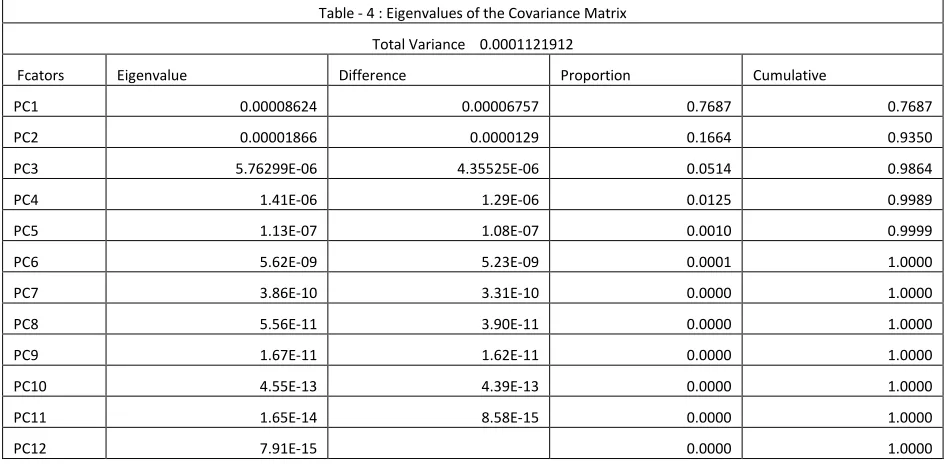
PCA has been applied to the monthly yield changes data from Apr’99 to May’12 for the set of maturities discussed
in Section 2. Table – 4 gives the key factors of Indian yield curve changes. The table gives the eigenvectors and
eigenvalues of the covariance matrix of monthly changes in the Indian zero-coupon rates from April’99 through
[image:12.612.70.542.351.583.2]May’12.
Table - 4 : Eigenvalues of the Covariance Matrix Total Variance 0.0001121912
Fcators Eigenvalue Difference Proportion Cumulative
PC1 0.00008624 0.00006757 0.7687 0.7687 PC2 0.00001866 0.0000129 0.1664 0.9350 PC3 5.76299E-06 4.35525E-06 0.0514 0.9864
PC4 1.41E-06 1.29E-06 0.0125 0.9989
PC5 1.13E-07 1.08E-07 0.0010 0.9999
PC6 5.62E-09 5.23E-09 0.0001 1.0000
PC7 3.86E-10 3.31E-10 0.0000 1.0000
PC8 5.56E-11 3.90E-11 0.0000 1.0000
PC9 1.67E-11 1.62E-11 0.0000 1.0000
PC10 4.55E-13 4.39E-13 0.0000 1.0000 PC11 1.65E-14 8.58E-15 0.0000 1.0000
PC12 7.91E-15 0.0000 1.0000
The first three principal components explain a major part of the total variance of interest rate changes. This result
is consistent with other studies. The first factor accounts for 76.87% of the total variance, while the second and
third factors account for 16.64% and 5.14%, respectively. In sum, the first three principal components explain
98.64% of the variability of the data, which indicates that these factors are sufficient for describing the changes in
the term structure in India. Chart – 5 shows the shape of the eigenvectors corresponding to the first three principal
[email protected] 12
principal component on the term structure of interest rates. The change in the zero-coupon rates is plotted against
the maturity terms with respect to each principal component. The first principal component basically represents a
parallel change in yield curve, which is why it is usually named the level or the height factor. The second principal
component represents a change in the steepness, and is named the slope factor. The third principal component is
called the curvature factor, as it basically affects the curvature of the yield curve by inducing a butterfly shift
(Nawalkha, Soto and Beliaeva).
An unit change of the ith factor cause a change ajt for each maturity t-year rate. Since factors are independent of
each other, we may therefor express the total change of the random variable rt by
∑
where fj is the j th
factor, k is the number of factors, ajt is the coefficient, identified by eigenvector analysis, used to
approximate the variance.
Our results show the coefficients for factor 1 is always positive, for factor 2, it is negative at start but turns to
positive and for factor 3, it starts with negative values, then positive in the middle part of maturity and then turns
to negative at the en part of the yield curve. -0.5000
-0.4000 -0.3000 -0.2000 -0.1000 0.0000 0.1000 0.2000 0.3000 0.4000 0.5000
0 5 10 15 20 25 30
Fact
o
r
Load
in
g
(%
)
Maturity (Years)
Chart - 5: Impact of Three most significant Components on Yield Curve
[email protected] 13
Table - 5: Eigenvectors of 3 Principal Components Eigenvectors
Maturity PRIN1 PRIN2 PRIN3
0.25 0.3520 -0.4447 -0.3446 0.5 0.3387 -0.4069 -0.2010
1 0.3173 -0.3396 0.0261
2 0.2897 -0.2289 0.3014
5 0.2622 -0.0013 0.4681
7 0.2598 0.0944 0.3979
10 0.2616 0.1865 0.2492
12 0.2637 0.2261 0.1520
15 0.2671 0.2659 0.0211
20 0.2726 0.3027 -0.1582
25 0.2777 0.3209 -0.2997
30 0.2824 0.3299 -0.4140
The result shows that a1,10 as 0.2616 implying a unit change in factor 1 causes 0.2616 change in 10-year rate – if the
10-year rate is 8.50%, then it will become 8.52% due to a level factor change of 1 unit. For all factors, it will change
to (0.2616%+0.1865%+0.2492% = 0.6973%) 8.56%.
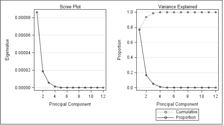
A scree plot is a plot of the Eigenvalues against the number of factors in order of extraction. Experimental
evidence indicates that the point at which the scree begins denotes the true number of factors. Generally, the
number of factors determined by a scree plot will be one or a few more than that determined by the Eigenvalue
criterion. The examination of the Scree plot provides a visual of the total variance associated with each factor. The
steep slope shows the large factors. The gradual trailing off (scree) shows the rest of the factors usually lower than
an Eigen value of 1. In choosing the number of factors, in addition to the statistical criteria, one should make initial
decisions based on conceptual and theoretical grounds. At this stage, the decision about the number of factors is
[email protected] 14
6. Conclusion
Principal Component Analysis has been widely used to study the shift in the term structure of interest rate. We
have used PCA to identify the factors which are responsible for changes in yield curve. The results indicate that the
three factors provide us the most of the variations in the term structure shift in India market. The study finds that
the first three principal components explain a major part of the total variance of interest rate changes. This result
is consistent with other studies. The first factor accounts for 76.87% of the total variance, while the second and
third factors account for 16.64% and 5.14%, respectively. In sum, the first three principal components explain
98.64% of the variability of the data, which indicates that these factors are sufficient for describing the changes in
the term structure in India.
References
Adrian, T., and H. Wu (2009): “The Term Structure of Inflation Expectations,” Working Paper, Federal Reserve Bank of New York.
Ang, A., J. Boivin, S. Dong, and R. Loo-Kung (2010): “Monetary Policy Shifts and the Term Structure,” Review of Economic Studies, forthcoming.
Buraschi, A., A. Cieslak, and F. Trojani (2010): “Correlation Risk and the Term Structure of Interest Rates,” Working paper, University of Lugano.
Campbell, J. Y., A. Sunderam, and L. M. Viceira (2011): “Inflation Bets or Deflation Hedges? The Changing Risk of Nominal Bonds,” Working paper, Harvard Business School.
Chan, K. C., G. A. Karolyi, F. A. Longstaff, and A. B. Sanders (1992): “An Empirical Comparison of Alternative Models of the Short-Term Interest Rate,” Journal of Finance, 47, 1209–1227.
Cieslak, A., and P. Povala (2011): “Understanding Bond Risk Premia,” Working Paper, Northwestern University and University of Lugano.
Cox, J. C., J. E. Ingersoll, and S. A. Ross (1985): “A Theory of the Term Structure of Interest Rates,” Econometrica, 53, 373–384.
Fleming, M. J. (1997): “The Round-the-Clock Market for U.S. Treasury Securities,” FRBNY Economic Policy Review.
Fontaine, J.-S., and R. Garcia (2011): “Bond Liquidity Premia,” Review of Financial Studies, forthcoming.
Haubrich, J., G. Pennacchi, and P. Ritchken (2011): “Estimating Real and Nominal Term Structures using Treasury Yields, Inflation, Inflation Forecasts, and Inflation Swap Rates,” Working Paper, Federal Reserve Bank of Cleveland.
Hautsch, N., and Y. Ou (2008): “Yield Curve Factors, Term Structure Volatility, and Bond Risk Premia,” Working paper, Humboldt Univeristy Berlin.
Hu, X., J. Pan, and J. Wang (2011): “Noise as Information for Illiquidity,” Working paper, MIT Sloan School of Management.
[email protected] 15
JP Morgan (2011): “The Domino Effect of a US Treasury Technical Default,” US Fixed Income Strategy, April 19, 2011.
Kim, D. H., and K. J. Singleton (2011): “Term Structure Models and the Zero Bound: An Empirical Investigation of Japanese Yields,” Working Paper, Yonsei University and Stanford University.
Litterman, R., Scheinkman, J. (1991). Common factors affecting bond returns. Journal of Fixed Income, Vol. 1, pp. 54–61.
Mishkin, F. (2006), The Economics of Money, Banking and Financial Markets, Addison-Wesley.
Nath, Golaka C., Yadav, Gaurav and Wagle, Amruta (2006), Estimating A Reliable Benhcmark Sovereign Yield Curve in an Emerging Bond Market (CCIL)
Nelson, Charles R. and Siegel, Andrew F., Parsimonious Modeling of Yield Curves. Journal of Business, 60(4):473– 489, 1987.
Phoa, W. (1997): “Can You Derive Market Volatility Forecast from the Observed Yield Curve Convexity Bias?,” Journal of Fixed Income, pp. 43–53.