Common factors and specific factors

Munich Personal RePEc Archive

Common Factors and Specific Factors

Chen, Pu

Melbourne Insitute of Technology

20 January 2012

Online at

https://mpra.ub.uni-muenchen.de/36114/

Common Factors and Specific Factors

Pu Chen

20.01.2012

Abstract

In this paper we study factor models for security returns on financial mar-kets, where some pervasive factors are common across all securities and other pervasive factors prevail only within some groups of securities but not in others. This kind of structured factors allow a more nuanced analysis of de-terminants of the security returns, in particular, they allow to study clustering structures in security returns as well as their determinants. The clustering structure provides a natural way to group the securities and to interpret com-mon factors and group-specific factors. We give conditions under which the common factor space and the group-specific factor spaces can be identified, and propose an effective procedure to estimate the unobservable structure in the factor space. Concretely, the procedure will determine the unknown ber of groups, endogenously classify securities into groups, determine the num-ber of common factors across all groups as well as the numnum-ber of group-specific factors in each group, and estimate the common factors and the group-specific factors. The estimated factor structure will provides a more meaningful in-terpretation of the estimated factors in practical applications.

KEYWORDS: Factor Models, Generalized Principal Component Analysis, Mul-tiset Canonical Correlation

JEL Classification: C63, G10, G12,

1

Introduction

The arbitrage pricing theory (ATP) of Ross (1976) provides a theoretically founded multifactor model for asset pricing. A key feature of the APT is that the random returns of each asset are assumed to be driven by a linear combination of a small number of common factors and an asset-specific random factor. The asset specific factor called idiosyncratic factor is assumed to be independent across all assets1_.

A series of statistical procedures (see Chapter 6 in Campell, Lo, and Mackenlay (1997)) have been developed to carry out empirical investigations based on APT. A large body of empirical literature on APT documents the success of APT.

APT maintains the possibility that some common factors that are pervasive across all assets, while some other pervasive factors prevail only within a group of assets. Group-specific factors are particularly useful in understanding data of the groups. So, industrial indices that are considered as industry-specific factors are used to measure industry-specific risks that can in turn explain the asset returns in re-spective industries (See Fama and French (1993) for more details.). In characteristic-based factor models it becomes a common practice to use industry-country factors as group-specific factors (see L. and Rouwenborst (1994)). In statistical factor models treatments of grouped data have a long tradition. Classic methods of factor rota-tion2 _{can be seen as procedures that implicitly seeking for some kinds of grouped}

structures in factor spaces. By discovering a ”simple structure” in the factor space, variables are divided accordingly into groups at the same time. In the literature there are also works that explicitly study grouped data in statistical factor models. Krzanowski (1979) considers the situation in which the group-specific factor spaces and the common factor space are the same and proposed to determine the com-mon factor space by minimizing its angles to the group-specific factor spaces. Flury (1984) and Flury (1987) consider the case in which all group-specific covariance ma-trices can be orthogonalized by a same matrix. This method is then extended by Schott (1999) to take into account of the situation in which the group-specific factor spaces are only subspaces of the common factor space respectively. He suggests to estimate the common factor space by applying principal components method to the sum of the eigenprojection of each group. Goyal, Perignon, and Villa (2008) apply this method to study the asset returns in NYSE and NASDAQ and find that these two markets share one common factor and each market has one group-specific factor respectively.

In the papers on grouped factor models listed above, the most important model parameters of the grouped structure: the number of groups, the membership rela-tions between groups and variables are assumed to be known a priori rather than estimated from observed data. In many cases even the numbers of common factors and group-specific factors are also given a priori. An attempt that assumes the grouped structure is unknown and estimates it from observed data is given in Chen (2010). The author applies the method of generalized principle component analy-sis to classify the variables into their groups and uses an information criterion to determine the number of groups and number of factors in each groups. After the

1_{Cross-sectional independence is required only in exact factor models. In approximate factor}

models the independence assumption is replaced by an assumption that the idiosyncratic factors are diversifiable.

2_{See for instance Kaiser (1958) and Johnson and Wichern (1992) Chapter 9 for more details on}

classification of variables into groups group-pervasive factors are estimated group by group using the standard principal component method.

The procedure in Chen (2010) provides however no inference on common factors and group-specific factors, which are among main interests in studying a grouped factor model. In this paper we extend the procedure in Chen (2010) to estimate the common factors and group-specific factors. Concretely, we apply the method of multiset canonical correlation analysis to extract the common factors from the estimated group-pervasive factors resulted from the procedure in Chen (2010). Then we subtract the common component due to common factors from data and apply the principal component method to the data net the common component to obtain an estimate of the group-specific factors. This method works only when we subtract the right common component due to the common factors from the data. For this reason we develop a consistent model selection criterion to determine the number of common factors and the number of group-specific factors in each group. Our paper contributes to the literature on factor analysis in that it provides a coherent method to explore structures in an unobservable factor space. The method will determine the number of groups, endogenously classify variables into groups, determine the number of common factors and the number group-specific factors in each group, and give consistent estimates of the common factor space and the group-specific factor space.

The paper is organized as follows. In section 2 we defined a grouped factor model with explicitly formulated common factors and group-specific factors. In section 3 we present a procedure to estimate common factors and group-specific factors. Section 4 presents simulation studies on the estimation procedure. Last section concludes.

2

The Model

Let X be a (T _×N) matrix collecting observations of a set of N security returns observed overT periods. We assume that this set of securities consists of n groups:

X

(T×N)= (TX1×N1

, X2

T×N2

, ...., Xn T×Nn

), with N =

n

∑

i

Ni. (2.1)

Further we assume that the return generating process for groupihas a factor struc-ture as follows.

Xi,jt

(1×1)

= Fi,t

(1×ri) ′ _λ

i,j

(ri×1)

+ ei,jt

(1×1)

, for i= 1, ..., n;j = 1, ...Ni;t = 1, ..., T; (2.2)

where Xi,jt is the return of the j-th security in the i-th group at time t, Fi,t is an

ri-vector of unobservable factors in the i-th group at time t, λi,j is an ri-vector of

factor loadings,riis the number of factor in theith group andei,jtis the idiosyncratic

component ofXi,jt. In matrix form, we have:

Xi

(T×Ni)

= Fi

(T×ri)

Λi

(ri×Ni)

+ Ei

(T×Ni)

, for i= 1,2, ..., n, (2.3)

where

• Xi: (T ×Ni) matrix collecting observations of Ni security returns in the ith

• Fi = (Fi,1, Fi,2, ..., Fi,T)′: (T ×ri) matrix containing ri unobservable

group-pervasive factors of the ith group over T periods.

• Λi = (λi,1, λi,2, ..., λi,Ni): (ri × Ni) matrix of unobservable group-pervasive

factor loadings of the ith group.

• Ei: (T ×Ni) matrix of unobservable idiosyncratic components of the Ni

secu-rity returns.

• ∑ni=1Ni =N.

In order to model common factors and group-specific factors explicitly, we assume that a small number, say rc_{, of pervasive factors are common across all groups and}

the other pervasive factors are only pervasive within some groups. We call the former common factors and the later group-specific factors. Since factors and loadings are identified up to a full rank transformation, we can assume with loss of generality that the common factors and the group-specific factors are uncorrelated in each group. This leads to the following formal assumption.

Assumption 2.1

(a) Group-pervasive factors in each group consist of rc _{common factors F}c t and a

set of rs

i group-specific factors Fi,ts.

Fi,t

(ri×1)

=

( Fc

t

Fs i,t

)

((rc_+rs i)×1)

, for i= 1,2, ..., n,

with rc_+rs i =ri.

(b) The common factors and the group-specific factors are uncorrelated.

E(F_tc, F_i,ts′) = 0

(rc_×rs i)

, for i= 1,2, ..., n. (2.4)

We assume that all common factors have been included in Fc

t, so that under

As-sumption 2.1 (a) and (b) the common factor space is identified. In terms of the common factors and the group-specific factors, the grouped factor model (2.3) can be rewritten as

Xi,jt

(1×1)

= F_tc′ (1×rc₎

λc_i,j (rc_×1)

+ F_i,ts′ (1×rs i)

λs_i,j (rs

i×1)

+ ei,jt

(1×1)

, for i= 1,2, ..., n, (2.5)

where λc

i,j and λsi,j are the loadings corresponding to the common factors and the

group-specific factors with (λc′

i,j, λs

′

i,j)′ =λi,j. In matrix form we have:

Xi

(T×Ni)

= Fc (T×rc₎ Λ

c i

(rc_×N i)

+ F_is (T×rs

i)

Λs_i

(rs i×Ni)

+ Ei

(T×Ni)

, for i= 1,2, ..., n, (2.6)

where Fc _{= (F}c

1, F2c, ..., FTc)′, Λci = (λci,1, λci,2, ..., λci,Ni), F

s

i = (Fi,s1, Fi,s2, ..., Fi,Ts )′ and

Λs

i = (λsi,1, λsi,2, ..., λsi,Ni). We called model (2.6) a grouped factor model with common

If group-specific factors are linearly independent across all groups, the union of the group-specific factor spaces will be rs_{-dimensional with r}s ₌ ∑n

i=1ris.

Col-lecting all group-specific factors together, we have Gs

t = (F1s,t′, F2s,t′, ..., Fn,ts ′)′ and

subsequently each group-specific factor Fs

i,t can be represented as a linear function

ofGs

t. If some components of a group-specific factor are exactly linearly dependent

on those of other groups, the dimension of the union of the group-specific factor spaces, say Ks_{, will be less than} ∑n

i=1ris. In fact, the dimension of the union will

be the number of all linearly independent components of the group-specific factors over all groups. Let a Ks_{-dimensional vector F}s

t collect all these linearly

indepen-dent components of the group-specific factors of all groups, then each group-specific factor Fs

i,t can be represented as a linear function of Fts. Therefore, we make the

following assumption.

Assumption 2.2

(a) Group-specific factor Fs

i,t is a linear function of a Ks dimensional factor Fts

with Ks_≤∑n

i=1ris in the following way:

Fs

i,t =Cis′Fts, for i= 1,2, ..., n. (2.7)

where Cs

i is a (Ks×rsi) constant matrix.

(b) rank(Cs

i) =rsi.

(c) rank(Cs

1, C2s, ..., Cns) = Ks.

While we assume that the common factors and the group-specific factors are un-correlated, we allow correlations and linear dependence among the group-specific factors across groups. This is included in Assumption 2.2 (a): If Ks _< ∑n

i=1ris,

group-specific factors will be linearly dependent across groups. For instance, with

n= 3, rc _{= 2, r}s

1 = 2 and r2s = 2, rs3 = 1 and Ks = 3 we are considering a grouped

factor model with three groups. All three groups share two common factors; each of the three groups has two, two and one group-specific factors respectively; and the five group-specific factors are located in a three dimensional specific factor space, such that these group-specific factors must be linearly dependent across the three groups. Assumption 2.2 (b) is made to ensure that with in a group the group-specific factors are not linearly dependent, such that no components of a group-specific fac-tor are redundant. (c) is to make sure that every component of the facfac-torFs

t is used

in generating the group-specific factors.

In order that each group is identified, no group-specific factor space of one group can be a subspace of that of another group, in other words Fs

i,t must not be a

lin-ear function of Fs

j,t: formally Fi,ts ̸= C′Fj,ts for any constant matrix C. Because

Fs

i,t = Cis′Fts and Fj,ts = Cjs′Fts, we will require that Cis ̸= CjsC for any constant

matrix C. This excludes in particular the possibility that Fs

i,t is just a rotation of

Fs

j,t. Further, since groups are characterized through their data points, we want

be different3_{. This leads to the following assumption.}

Assumption 2.3

(a) Cis and Cjs are not linearly dependent, i.e. Cis̸=CjsC, for any constantC with

i_̸=j, i= 1,2, ..., n and j = 1,2, ..., n.

(b) Any pair of loading vectors of different groups λs

i,m and λsj,l for m= 1,2, ...Ni,

l = 1,2, ..., Nj, i= 1,2, ..., n, j = 1,2, ..., n and i̸=j satisfy the restriction:

Cs

iλsi,m ̸=Cjsλsj,l.

Assumption 2.3 (a) says no group-specific factors are linear combinations of those of another group. In the case with two specific factor planes and one group-specific factor line mentioned earlier, this assumption excludes the situation in which the line lies on either of the two planes and the situation where one plane lies on the other, so that the three group-specific factor spaces are different. Assumption 2.3 (b) excludes the situation in which a data point is located around the intersection of the factor spaces of two groups4_{, such that the relationship between variables and}

groups is unambiguously defined. The common factors Fc

t and the specific factors Fts constitute an (rc +Ks)

di-mensional overall pervasive factor space. We used an (rc_+Ks_{) dimensional vector}

Ftp =

( Fc

t

Fs t

)

to represent the overall pervasive factors5_{. Then, following}

Assump-tion 2.2, each group-pervasive factorFi,t can be written as a linear function of Ftp.

Fi,t =

( Fc

t

Fs i,t

)

=

(

I 0

0 Cs i′

) ( Fc

t

Fs t

)

=C_i′Ftp, for i= 1,2, ..., n, t= 1,2, ..., T,

(2.8)

with C′

i =

(

I 0

0 Cs i′

)

. Denoting Fp _{= (F}p

1, F

p

2, ..., F

p

T)′, we can present equation

(2.8) in a matrix form: Fi =FpCi.

Under Assumptions 2.1 to 2.3, the polled security returns X adopts a factor structure with Fp _{as the factors:}

X = ( X1 X2 . . . Xn

)

= ( F1Λ1 F2Λ2 . . . FnΛn

)

+( E1 E2 . . . En

)

= ( Fp_C1Λ

1 FpC2Λ2 . . . FpCnΛn

)

+( E1 E2 . . . En

)

= Fp( C1Λ1 C2Λ2 . . . CnΛn

)

+( E1 E2 . . . En

)

3_{This is a technical assumption to simplify the presentation of a correct classification. Without}

this assumption we may have situations in which some data points may belong to more that one group. which will complicate a definition of correct classification.

4_{This is a technical assumption to simplify the presentation of a correct classification of variables.}

However, this assumption is not essential for estimation of the structured factor space. See Chen (2010) for more details.

5_{Note that Assumption 2.1 (b) allows us a simple presentation of the overall pervasive factor}

as combination ofFtp= (Fc

′

t , Fs

′

t )′. Without this assumptionF p

t will be a basis of the union space ofFc

Defining Λ = (C1Λ1, C2Λ2, ..., CnΛn) and E = (E1, E2, ..., En), we have:

X

(T×N)= F

p

(T×K)(KΛ×N)+(TE×N) (2.9)

The equation above says that X can be accommodated in an ungrouped factor model with K =rc_+Ks _factors.

Benefits of studying the grouped factor model (2.6) instead of the pooled un-grouped factor model (2.9) are that the un-grouped factor model provides a more de-tailed information on the data as well as the data-generating process. In stead of saying that all variables are influenced byK factors, we can say the variables consist ofngroups and there arerc _{common factors that influence all variables. In addition}

variables in each group is influenced by additional ks

i group-specific factors. This

detailed specific information can be used in association with possible group-specific structural information to provide a better interpretation of the factors.

In order to apply the estimation procedure given in Chen (2010) we adopt the model assumptions on factors and factor loading from Bai and Ng (2002), which is also applied in Chen (2010).

Assumption 2.4

E_||Ftp||4 <∞ and E||√1_T

∑T t=1(F

p

tFtp′ −E(FtpFtp′))|| < M as T → ∞. Denote the

positive definite matrixE(FtpFtp′) by Σp.

Assumption 2.5

||λi,j|| < λ < ∞ and ||ΛiΛ′i/Ni −Li|| → 0 as Ni → ∞ for some (ri ×ri) positive

definite matrix Li, for i= 1,2, ..., n.

LetXjt denote the observation of thejth variable at timet inX and ejt be the

idiosyncratic component ofXjt in the ungrouped model (2.9).

Assumption 2.6 (Time and Cross-Section Dependence and Heteroskedasticity)

There exists a positive constantM _{≤ ∞}, such that for all N and T, 1. E(ejt) = 0, E|ejt|8 ≤M;

2. E(∑N_j=1ejsejt/N) = γN(s, t),|γN(s, s)| ≤M for all s, and

T−1∑T

t=1 ∑T

s=1|γN(s, t)| ≤M;

3. E(ejtekt) =τjk,twith|τjk,t| ≤ |τij|for someτjk and for allt,N−1∑N_j=1∑N_k=1|τjk|<

M

4. E(ejteks) =τjk,ts and (N T)−1∑Nj=1 ∑N

k=1 ∑T

t=1 ∑T

s=1|τjk,ts| ≤M,

5. for every(t, s), E_|N−1/2∑N

i=1[ejsejt−E(ejsejt)]|4 ≤M.

Further we adopt also the assumption on weak dependence between factors and errors given in Bai and Ng (2002).

Assumption 2.7 (Weak Dependence between Factors and Errors)

E (

1

N

N

∑

j=1

1 √

TF

p tejt

2)

Assumption 2.4 is to a certain degree a strong assumption in a factor model. A standard assumption such as in Bai and Ng (2002) requires only law of large number type convergency: _T1 ∑T_t=1FtpFtp′

P

−→ Σp_{. We require instead a stronger condition}

E_||√1

T

∑T t=1(F

p tF

p

t′−Σp)||< M. However, for practical application purposes, these

two kinds of assumptions make no essential difference.

Under Assumption 2.2 and Assumption 2.4 it is easy to see that the group-pervasive factorFi,t also satisfies the requirements of Assumption 2.4, i.e.

(1) E_||Fi,t||4 =E||Ci′F p

t||4 <∞

(2) _T1 ∑T_t=1Fi,tFi,t′ = _T1 ∑Tt=1CiFtpFtp′Ci′ P

−→CiΣpCi′ as T → ∞. Since rank(Ci) =

ri =rc+ris, CiΣpCi′ is a positive definite matrix.

Assumption 2.5 is to make sure that each component of a group-pervasive factor makes a nontrivial contribution to the variance of the variables in the group.

Proposition 2.8

Under Assumption 2.5 and Assumption 2.2 (d) and (e), the factor loading matrix

Λ in the ungrouped model (2.9) satisfies the requirement in Assumption 2.5, i.e.

||λj|| < λ < ∞ and ||ΛΛ′/N − L|| → 0 as N → ∞ for some (K ×K) positive

definite matrix L.

Proposition 2.9

(a) rank(Ci) = ri =rc+rsi.

(b) rank(C1, C2, ..., Cn) = K.

(c) K _≤rc₊∑n i=1rsi.

This proposition follows the assumption that the common factors and the group-specific factors are uncorrelated. Comparing model Assumptions 2.1 through 2.7 with the model assumptions given in Chen (2010), we know that our group factor models with common factors here satisfy all the assumptions on grouped factor models given in Chen (2010). Therefore, group factor models with common factors belong to a special class of grouped factor models with explicitly defined common factors and group-specific factors.

3

Estimation of Factors

In studying grouped factor models with common factors given in (2.6), instead of assuming that the number of groups, the membership relation between securities and their respective groups are knowna priori, we want to estimate them from observed data. In other words, determination of the number of groups, classification of the securities into their respective groups, and estimation of the common factors and the group-specific factors are objectives in this paper.

3.1

Estimation of Group-pervasive Factors

number of the group-pervasive factors and estimate group-pervasive factors for each group. We restate the estimation procedure briefly as follows.

• Step 1: Estimate the dimension of the overall pervasive factor spaceK by the

P C criterion of Bai and Ng (2002).

• Step 2: Project the (T _×N) data matrixX onto a (K _×N) matrix:

¯

XT = 1

TFˆ

K′

X,

where ˆFK_{is a principal component estimator ofF}p_{with ˆF}K ₌ 1

N T(XX′)

√

T Q, where Q is a (T _×K) matrix containing K eigenvectors corresponding to the

K largest eigenvalues ofXX′_.

• Step 3: According to a set of chosen model parameters (n,_{ki}ni=1), solve

the classification problem for the projected data by polynomial differentiation algorithm with voting scheme

• Step 4: Use the model selection criterion to evaluate alternative choices of models to obtain an optimal model (ˆn,_{ˆki}niˆ=1) and the corresponding

classifi-cation of variables _{Xsn

i }niˆ=1.( Xisn represents the securities classified into the

ith group.)

• Step 5: Estimate a factor model for each group of data in_{Xsn

i }niˆ=1by the

prin-cipal component method to obtain estimates for the respective group-pervasive factors ˆFi = _N1_iT(XisnXisn′)

√

T Qi, whereQi contains the ˆki eigenvectors

corre-sponding to the ˆki largest eigenvalues of the matrix XisnXisn′.

It is shown that this procedure will achieve a consistent classification of the securities into their respective groups. The procedure gives also consistent estimates of group-pervasive factor space for each group.

What we want particularly to focus on in this paper is to estimate the com-mon factors and the group-specific factors in a grouped factor model. A question raises naturally: can we directly derive estimates for the common factors and the group-specific factors from the estimates of the group-pervasive factors? In some circumstances the answer is positive. Let’s denote a grouped factor model by the numbers of factors in each group and the dimension of the overall pervasive factor space: [r1, r2, ..., rn|K]. For example [2 2| 3] indicates a grouped factor model with

For instance the factors in the three groups can be: ([F1F2][F2F3][F3F4]) in which the first two groups share one factor F2 and group 2 and group 3 share one factor F3 and the three groups do not have any common factors. In this case none of the three canonical variables can be used as an estimate of the common factor.

Generally the information on the group-pervasive factors estimated group by group are not directly conclusive for the common factor space and the group-specific factor spaces. We need a more detailed study in order to obtain an estimate for the common factors. In the next subsection we will present a procedure to estimate the common factors and the group-specific factors as well.

3.2

Estimation of Common Factors and Group-Specific

Fac-tors

Multiset canonical correlation analysis is extends the canonical correlation analysis between two groups to more groups6_{. It targets at finding linear combinations in each}

group, such that the correlations among these linear combinations are maximized across all groups. SinceFc

t are the common factors among all group-pervasive factors

Fi,tfori= 1,2, ...n,the firstrcmultiset canonical variables across all group-pervasive

factors must be the common factors or linear combinations of the common factors. Let Σij denote the covariance matrix between the group-pervasive factors of

the ith group and those of the jth group: Σij = E(Fi,tFj,t′ ), the calculation of

the multiset canonical correlation coefficients is to solve the following maximization problem:

max

ai,aj

tr

( _n ∑

i=1

n

∑

j=1

(a′_iΣijaj)

)

= max

ai,aj

tr

( _n ∑

i=1

n

∑

j=1

E(a′_iFi,t, a′jFj,t

) )

(3.10)

s.t. a′_iΣiiai =Irc. for i= 1,2, ...n. (3.11)

where ai and aj are (ri ×rc) and (rj ×rc) matrices. a′iFi,t and a′jFj,t represent rc

linear combinations of the pervasive factors in groupiand groupj respectively. The motivation of this maximization problem explains itself. The objective function is the sum of pairwise canonical correlation coefficients over all groups. The restrictions in (3.11) is to make sure that the summands in the objective function are properly normalized to be canonical correlation coefficients.

Collecting Fi,t, ai, and Σij over all groups into (∑ni=1ri×1), (∑ni=1ri×rc) and

(∑n_i=1ri×∑ni=1ri) matrices respectively, we obtain:

Ft=



 

F1,t

...

Fn,t



 , a=



 

a1

...

an





, and Σ = 

 

Σ11 . . . Σ11

... ... ... Σn1 . . . Σnn





, so that the

maximiza-tion problem (3.10) can be written in the following matrix form:

max

a

tr (a′Σa) (3.12)

s.t. a= (a′

1, a′2, ...a′n)′, and a′iΣiiai =Irc. fori= 1,2, ...n. (3.13)

wherea is a ((∑n_i=1ri)× rc) matrix.

6_{See Nielsen (2002) and Hasan (June 2009) for more details on multiset canonical correlation}

Since all group-pervasive factors share rc _{common factors, the common factors}

must be the canonical variables, i.e. we can calculate the common factors as follows:

Fc t = n1

∑n

i=1a′iFit = _n1a′Ft, whereais a solution of the maximization problem (3.12).

In order to overcome the difficulties of local maxima and to make the compu-tation more efficiently, we reformulate the nonlinear optimization problem (3.12) under restriction in (3.13) into an eigenvalue problem through standardizing the group-pervasive factors. Defining F∗

it = Σ

−1 2

ii Fi,t, we have Σ∗ij = E

( F∗

itF∗

′

ji

)

=

E(Σ− 1 2

ii FitFji′Σ

−1 2

jj

)

= Σ− 1 2

ii ΣijΣ−

1 2

jj , and Σ∗ii = V ar(Fit∗) = Iki. Stacking Fi,t∗ over

all groups, we have F∗′

t = (F∗

′

1,t, F∗

′

2,t, ..., F∗

′

n,t) and Σ∗ = E(Ft∗F∗

′

t ). Then the

maxi-mization problem (3.12) can be reformulated as follows:

max

a

tr (a′Σ∗a) (3.14)

s.t. a′ = (a1, a2, ...an)′, and a′iai =Irc. for i= 1,2, ...n. (3.15)

Being multiset canonical variables, the standardized common factors can be cal-culated as follows: Fc∗

t = n1

∑n i=1a

′

iFit∗ = n1a′Ft∗, where a is the solution of the

maximization problem (3.14). The maximization problem (3.14) differs from the following problem:

max

a tr (a

′_Σ∗_{a) (3.16)}

s.t. a′a=nIrc, (3.17)

only in that thenrestrictions in problem (3.15) are replaced by one single restriction on the sum of then restrictions: a′_a=∑n

i=1a′iai =nIrc in (3.17). It is well known

that the maximization problem (3.16) under (3.17) is an eigenvalue problem (See Johansen and Wichern (1992) p. 459): the solution are the eigenvectors of length √

n corresponding to therc _{largest eigenvalues. Because the maximization problem}

in (3.16) relaxes the restrictions in the maximization problem in (3.14), generally the two problems will have different solutions. However, in our case the Σ∗ _{matrix has a}

particular structure, such that it can be shown that these two problems have identical solutions. Therefore we can solve the problem (3.14) via solving the eigenvalue problem (3.16). We summarize this fact in the following proposition.

Proposition 3.1

Under Assumptions 2.1 to 2.4

(i) Σ∗ _{has K nonzero eigenvalues.}

(ii) The first rc _{largest eigenvalues of Σ}∗ _{are identical and their value is n. The}

length-√n eigenvectors that correspond to therc _{largest eigenvalues of Σ}∗ _solve

the maximization problem (3.16) and they solve the maximization problem (3.14) as well.

(iii) There exists a particular set of eigenvectors arc (see below) corresponding to

the first rc largest eigenvalues of Σ∗, such that Ftc∗ = √1na′rcF_t∗.

a′_rc =

1 √

n((rcI_×rc_rc₎ , 0

(rc_×rs

1)

, Irc

(rc_×rc₎ , 0

(rc_×rs

2)

, ..., Irc

(rc_×rc₎ , 0

(rc_×rs n)

(iv) The rc_{+ 1 to k}c _(rc _{< k}c _{≤ K) largest eigenvalues of Σ}∗ _{are nonzero and the}

corresponding eigenvectors denoted by aps _{has the property that √}1

na ps′

F∗

t spans

a subspace of the standardized specific factor space and hence also a subspace of the specific factor space. We denote _√1

na ps′

F∗

t by F ps∗

t .

aps′ = ( 0_rc

(krc_×rc₎ , aps₁ ′

(krc_×rs

1)

, 0_rc

(krc_×rc₎ , aps₂ ′

(krc_×rs

2)

, ..., 0_rc

(krc_×rc₎ , aps_n′

(krc_×rs n)

),

with _krc _=kc_−rc.

Comments:

Because the first rc _{largest eigenvalues of Σ}∗ _{are identical, obviously, any}

or-thogonal transformations of arc are still eigenvectors corresponding to the same

eigenvalues. The rc_{+ 1 to k}c _(rc _{< k}c _{≤K) largest eigenvalues of Σ}∗ _{are positive.}

Whether these eigenvalues are unique or not depends on data generating models, in particular, it depends on the relationship between the group-specific factors across groups. Because our main focus is not on the relations among the group-specific factors, we make an auxiliary assumption on the uniqueness of the rc _{+ 1 to k}c

(rc _{< k}c _{≤K) largest eigenvalues of Σ}∗_{, in order to simplify the presentation.}

Assumption 3.2

Therc+ 1 to kc (rc < kc _≤K) largest eigenvalues of Σ∗ are unique.

Under this assumption the corresponding eigenvectors aps _{are unique if we require}

that the first non-zero element in each column of aps _{is positive.}

Proposition 3.1 establishes that we can calculate the standardized common fac-tors and henceforth an estimate of the space of the common facfac-tors using the eigen-vectors of Σ∗_.

F_tc∗ = _√1

na

′

rcF_t∗. (3.18)

Still, we cannot use (3.18) to estimate Fc∗

t directly, because we don’t know Ft∗.

However, through estimation of group-pervasive factors we have an estimate ˆF∗

i,t for

F∗

i,t and an estimate ˆΣ∗ij for Σ∗ij with ˆΣ∗ij = T1

∑T

t=1Fˆi,t∗Fˆ∗

′

j,t. Stacking ˆFi,t∗ together

over all groups, we have ˆFt∗ = ( ˆF∗

′

1,t,Fˆ∗

′

2,t, ...,Fˆ∗

′

n,t)′ and ˆΣ∗ = T1

∑T

t=1Fˆt∗Fˆ∗

′

t .

Using ˆΣ∗ _{instead of Σ}∗_{, we can estimate the standardized common factors and}

hence the space of the common factors, by solving the following maximization prob-lem:

max

a

tr (a′Σˆ∗a) (3.19)

s.t. a′a=Irc. (3.20)

Obviously, the solutions of the maximization problem (3.19) are the unit length eigenvectors of ˆΣ∗ _{that correspond to the r}c _{largest eigenvalues of ˆΣ}∗_{. Denoting}

the solution of the maximization problem in (3.19) by ˆa, the rescaled canonical variable _√1

naˆ′Fˆt∗ serves as an estimate of the standardized common factors. If ˆa

and ˆF∗

t are consistent estimates of arc and F∗

t respectively, ˆFtc = √1naˆ′Fˆt∗ will be

on an assumption that we know the number of the common factors rc_{. If r}c _needs

to be determined, which is one of our objectives in this paper, we can only make a guess kc _{for r}c_{. If k}c _{< r}c _{the depicted procedure will lead to an estimate of only}

a subset of the common factor space; and if kc _{> r}c _{the procedure will lead to an}

estimate of a factor space containing the common factor space and a subspace of the specific factor space. We summarize this fact in the following theorem.

Theorem 3.3

Let kc _{be a guess of the number of the common factors with 0< k}c _{< r}

i and let the

(∑n_i=1ri)×kc matrix ˆhkc be eigenvectors corresponding to the kc largest eigenvalues

of Σˆ∗ _{and F}ˆc

t = √1nˆh′kcFˆ_t∗. Under Assumptions 2.1 to 2.7, for 1 ≤ kc ≤ rc, there

exists an (rc_×kc_{) matrix B}

rkc with rank(B_rkc) = kc, such that

1

T

T

∑

t=1

||Fˆ_tc ₋B_rk′ cF_tc||2 =O_p(C_N,T−2 ), (3.21)

with CN,T = min(

√

T ,√N); and for rc _{< k}c _{≤ K, there exists a (k}c_×kc_{) full rank}

matrix Bkc, such that

1

T

T

∑

t=1

Fˆtc −Bk′c

( Fc

t

Ftps

) 2

=Op(CN,T−2 ), (3.22)

where F_tps = √1

na ps′

F∗

t = √1n

∑n i=1a

ps′

i Σsi−

1 2Fs

i,t representing some (kc −rc) linear

combinations of the group-specific factors of all groups and aps _{is the matrix}

con-taining eigenvectors corresponding to therc_+1tokc _{largest eigenvalues ofΣ}∗ _defined

in Proposition 3.1 (iv).

Theorem 3.3 implies, in particular, that if we know the number of common factors, we can consistently estimate the space spanned by the common factors in the sense that the time average of the squared deviations between the estimated common factors and those lie in the true common factor space vanish asN, T _{→ ∞}. Because the common factorsFc

t can only be identified up to a rotation, we can only estimate

the space spanned by the common factors.

Now we turn to estimation of the group-specific factors Fs

i,t. We wish to have

observations on Xs

i =Xi−FcΛci =FisΛsi +Ei, because we could derive an estimate

for the group-specific factors fromXs

i that were generated only by the group-specific

factors. Xs

i is unfortunately unobservable. A natural estimate forXisis the residuals

of a linear regression ofXi on the estimate of the common factors ˆFtc:

Xi,jt = ˆFc

′

t ˆλci,j+ ˆXi,jtrs , i= 1,2, ...n;j = 1,2, ..., Ni, (3.23)

where ˆλc

i,j is the regression coefficient and ˆXi,jtrs is the regression residual. In matrix

form we have

ˆ

X_irs =Xi−Fˆc

′_ˆ

Λc_i, i= 1,2, ...n. (3.24)

The equation above says ˆXrs

i can be seen as data net the common components due

and idiosyncratic components. So we can apply the principal component method to the data of ˆXrs

i to obtain estimates of the group-specific factors group by group.

The strategy above works only when our guesskc _{is correct, i.e. k}c _=rc_{. Because}

rc _{is unknown, our guessk}c _{may differ fromr}c_{. For a choice of k}c _{we may potentially}

have three cases: (1) kc _{< r}c_{, (2) k}c _{= r}c _{and (3) k}c _{> r}c_{. According to Theorem}

3.3, for these three cases, ˆFc′

t may span different subsets of the pervasive factor

space and hence ˆFc′

t ˆλci,j may contain different parts of the common component.

Consequently, ˆXrs

i,jt = Xi,jt −Fˆc

′

t λˆci,j may have different influencing factors. For

kc _{< r}c_{, ˆX}rs

i,jt =Xi,jt−Fˆc

′

t ˆλci,j will contain more factors thanFi,jts , while forkc > rc,

ˆ

Xrs

i,jt =Xi,jt−Fˆc

′

t λˆci,j may contain fewer factors. Indeed, the number of the factors

that influence ˆXrs

i,jt depends on the choice of kc. The following proposition states

this fact formally.

Proposition 3.4

For a given choice of 0 < kc _{< r}

i, to the common factor estimate Fˆtc based on

Theorem 3.3 and the regression residuals Xˆrs

i,jt based on equation (3.23), there exit

population counterparts F_tpc and Xrs

i,jt, respectively, such that

(i) Xi,jt can be decomposed as:

Xi,jt =Fpc

′

t λ pc

i,j+Xi,jtrs

and Xrs

i,jt is generated by a factor model.

X_i,jtrs =F_i,trs′λrs_i,j +ei,jt.

(ii) Both F_tpc and the number of factors generating Xrs

i,jt, denoted by kirs, vary with

the choice of kc _{as follows:}

– for kc _{< r}c_{, F}pc

t = Brk′ cF_tc, with B_rkc an (rc × kc) matrix defined in

Theorem 3.3 and krs

i =rc−kc+rsi.

– for kc _=rc_{, F}pc

t =Br′cF_tc, X_i,jtrs =X_i,jts =Fs

′

i,tλsi,j+ei,jt and krsi =ris.

– For kc _{> r}c_{, F}pc

t = Bk′c

( Fc

t

Ftps

)

, where Bkc and F_tps are a (kc × kc)

matrix and a(kc_−rc_{)random vector defined in Theorem 3.3 respectively,}

and

∗ krs

i =rsi, if there is no exact linear dependence between Fi,ts and F pc t .

∗ krs

i =ris−kis∗, if there exits kis∗ linearly dependent relations between

Fs

i,t and F ps

t : Fi,ts′C = F ps

t ′B, where C is an (ris×ksi∗) matrix with

ks∗

i ≤ris and rank(C) = kis∗.

(iii) Let F˜s

i andFˆis be principal component estimates of factors based on the data of

(Xrs i Xrs

′

i )and on the data of( ˆXirsXˆrs

′

i ), respectively: F˜is = N1iT(X

rs i Xrs

′

i )

√

TQ˜ks i

with Q˜ks

i a (T ×k

s

i) matrix of the eigenvectors corresponding to the ksi largest

eigenvalues of (Xrs i Xrs

′

i )andFˆis = N1iT( ˆX

rs i Xˆrs

′

i )

√

TQˆks i with

ˆ

Qks

i is a (T×k

s i)

matrix of the eigenvectors that correspond to the ks

i largest eigenvalues of

( ˆXrs i Xˆrs

′

Then we have

1

T

T

∑

t=1

||F˜_i,ts ₋Fˆ_i,ts_||2 =Op(CN,T−2 ).

Proposition 3.4 (i) and (ii) imply in particular that for a correct guess ofkc_{, X}s i,t is

generated only by the group-specific factorsFs

i,t, so that we could obtain an estimate

for the group-specific factors from XisXs

′

i

NiT . (iii) states that the factor estimate based

on XˆirsXˆrs

′

i

NiT converges to the factor estimate based on

Xrs i Xrs

′

i

NiT . Therefore, we can use

the available XˆirsXˆrs

′

i

NiT instead of the unobservable

Xrs i Xrs

′

i

NiT to construct an estimate for

the group-specific factors. The following theorem states properties of the estimation based on XˆirsXˆrs

′

i

NiT . Theorem 3.5

For a given choice of (kc_{, k}s

i) satisfying 0 < kc < ri and 1 < kis, let Fˆtc be the

estimate of the common factors given in Theorem 3.3 and Xˆrs

i be residuals from

the regression in (3.24) and Fˆs

i be the estimate ofksi group-specific factors obtained

by applying the asymptotical principal component method to the data set of Xˆrs i :

ˆ

Fis =

ˆ

Xrs i Xˆrs

′

i

NiT

√

TQˆks

i, where Qˆksi is the eigenvectors corresponding to the k

s

i largest

eigenvalues of Xˆrsi Xˆrs

′

i

NiT . Under assumption 2.1 through 2.7, there exit a (k

c_×kc_{) full}

rank matrix_Hkc and a(ks_i×krs_i )full rank matrixH′_ks

i withrank(Hk s

i) = min(k

s i, krsi ),

such that

1

T

T

∑

t=1

||Fˆ_tc _{− H}′_kcF_tpc||2 =O_p(C_N,T−2 ), (3.25)

and

1

T

T

∑

t=1

||Fˆ_i,ts _{− H}′_ks iF

rs

i,t||2 =Op(CN,T−2 ). (3.26)

Combining (3.25) with (3.26), we have

1

T

T

∑

t=1

( _ˆ

Fc t

ˆ

Fs i,t

)

−

(

H′

kc 0

0 _H′

ks i

) ( F_tpc Frs i,t

) 2

=Op(CN,T−2 ). (3.27)

Denoting ( ˆFc′

t ,Fˆs

′

t )′ by Fˆt0, (F pc′

t , Frs

′

t )′ by Fˆt0 and diag(Hk′c,H′_ks

i) by H

0′

we can rewrite the equation above compactly as follows.

1

T

T

∑

t=1

||Fˆ_t0 _{− H}0′F_t0_||=Op(CN,T−2 ). (3.28)

Corollary 3.6

For kc _{= r}c _{and k}s

i ≥ 1, there exists an (ris×kis) matrix Hks

i with rank(Hkis) =

min(rs

i, ksi)7, such that

1

T

T

∑

t=1

||Fˆs

i,t− H′ks iF

s

i,t||2 =Op(CN,T−2 ), for i= 1,2, ..., n. (3.29)

7_H

ks

i matrix corresponds to theH

Theorem 3.3 and Corollary 3.6 establish that if we know the number of the common factors and the number of group-specific factors in each group, we can con-sistently estimate the common factor space as well as the respective group-specific factor spaces in the sense that the time average of the squared deviations between the estimated factors and those lie in the respective true factor spaces vanish as

N, T _{→ ∞}. Now a key question is how can we infer the number of the common fac-tors and the number of the group-specific facfac-tors in each group from data. Following the approach developed in Chen (2010), we are going to construct an information cri-terion to determine the number of common factors and the number of group-specific factors. Generally, an information criterion consists addictively of two terms: the likelihood of a model under consideration plus a penalty term due to the dimension-ality of the model. To ensure the consistence of the criterion, the penalty term must depend increasingly on the dimensionality of the model and converge at a slower rate than the likelihood term8_{. For this purpose we use the sum of squared residuals}

calculated as follows as the likelihood term of a group.

Vi(ksi,Fˆis|Fˆc, kc) = min_Λs i,,Fis

1

NiT Ni

∑

j=1

T

∑

t=1

[(Xi,jt−Fˆc

′

t ˆλci,j)−Fs

′

i,tλsi,j]2 fori= 1,2, ...n.

To take into account of the fact that common factors across all groups represent a more restrictive model than a model with the same numbers of group-pervasive factors, we need to put less penalty on the number of common factors than on the average number of group-specific factors.

The following theorem gives a concrete formulation of the penalty term and thus a consistent model selection criterion to determine the number of groups, the number of common factors and the numbers of group-specific factors as well.

Theorem 3.7

Let Xsn

i represent the data classified into ith group by the classification procedure

given in Chen (2010) and(kc_,{ks

i})represent a choice of the numbers of the common

factors and the group-specific factors in each group. Under Assumptions 2.1 through 2.7 a model selection criterion

C(n, kc,_{ks_i},_{Xsn

i }) = n

∑

i=1 Ni

NVi(k

s

i,Fˆis|Fˆc, kc) + ˆσ2(¯ks+ ¯h+αkc)g(N, T) (3.30)

is a consistent model selection criterion for a grouped factor model with common factors and group-specific factors, if the following additional conditions are satisfied:

1. limN→∞ NNi → αi, where Ni

N is the share of variables in the i−th group, αi >

α >0 and α= 1₋α. It is to note that α is the lower bound for all candidate models.

2. g(N, T)_→+0, C2

N,Tg(N, T)→ ∞ as N, T → ∞,

where CN T = min{

√

N ,√T_}.

3. h is a real valued function over (0,1) with the following properties: (a) 0< h(α)<1 for any 0_≤α_≤1

(b) h(αi)≥h(αj) for any 0≤αi ≤αj ≤1.

(c) ∑_lαlh(αl)>

∑

jαjh(αj) for and {αj}-{αl}.

We use the notation _{αj} - {αl} to present that {αj} is a finer partition of

the variables than _{αl}, with ∑_lαl = ∑_jαj = 1. h¯ = ∑n_i=1αih(αi) is the

weighted average of h(αi) over all groups.

Remarks

Compared to the criterion in Chen (2010), the likelihood term remains the weighted average of the sums of squared residuals over all groups. The criterion keeps the the penalty term ¯h due to dispersion of the groups. It modify the penalty term due to the average number of factor in that the number of common factors has a smaller penalty than the number of group-specific factors, reflecting the fact that one group-specific factor in each group gives more model flexibility than one common factor over all groups. Condition 1 is to make sure that the proportion of a group will not vanish asymptotically, Condition 2 is to get the right rate of convergence for the penalty term, and Condition 3 is to make sure that the average number of factors is the dominating parameter of the model and the dispersion of groups is a dominated parameter. While comparing two models, we compare first the dominating parameter, only when the dominating parameter are equal we compare the dispersion of the groups in the two models.

A concrete choice ofg(N, T) can be: • g(N, T) = N+T

N T log

( _{N T}

N+T

)

, and a concrete choice of h(Ni/N) is:

• h(ˆαi) =

ˆ

αiN+T

ˆ

αiNT log

( _ˆ

αiNT

ˆ

αiN+T

)

αN+T αN T log(

αN T αN+T)

= g( ˆαiN,T)

g(αN,T),

where ˆαi = N_Nj. Thish function is used in our simulation study.

3.3

Summary of the Estimation Procedure

• Step 1: Apply the procedure in Section 3.1 to obtain estimates of ˆn, ˆri and

ˆ

Fi,t for i = 1,2, ...,nˆ and calculate estimates of standardized group-pervasive

factors and covariance matrix ˆF∗

i,t, ˆFt∗ and ˆΣ∗.

• Step 2: Choose a set of proper model parameters (ˆn, kc_,{ks i}niˆ=1).

• Step 3: Calculate ˆFc _{= √}1 ˆ

nˆh′kcFˆt∗.

• Step 4: Regress Xi on ˆFc to obtain the regression residuals ˆXirs =Xi−FˆcΛˆi.

• Step 5: Estimate group-specific factors and the loadings using the data of ˆXrs i

for each group ˆFs

i = N1iT( ˆX

rs i Xˆrs

′

i )

√

T Qi,whereQicontains theksi eigenvectors

corresponding to the ks

i largest eigenvalues of the matrix ˆXirsXˆrs

′

i .

• Step 6: Calculate the model selection criterion values for alternative models

C(ˆn, kc,_{k_is_},_{Xsn

i }) =

ˆ

n

∑

i=1 Ni

NVi(k

s

i,Fˆis|Fˆc, kc) + ˆσ2(¯ks+ ¯h+αkc)g(N, T).

4

Simulation Studies and an Application

Exam-ple

4.1

Simulation Studies

The theoretical results presented in the last section can be used in two ways. If data are already available in grouped form, we do not need the classification step of the procedure in Section 3.3. The procedure can be used to determine the dimension of the overall pervasive factor space K and determine common factors across the groups and group-specific factors. If the existence of a grouped structure is only a working hypothesis and the groups need to be determined, the procedure in Section 3.3 will determine the number of groups, deliver a consistent classification of the variables and estimate the common factors and group-specific factors. Obviously, the performance of the estimation procedure for the former case can only be better than for the later case due the classification uncertainty involved in the later case. Therefore, we focus on a simulation study in the later case. If we have a satisfactory results here, we do not need to bother the performance in the former case.

The simulation study is conducted in order to assess the performance of the proposed estimation procedure in finite sample situations. In particular we want to assess the ability of the model selection criterion in identifying the true model, i.e. the number of groups and the number of common factors and the number of group-specific factors in each group. We use a vector consisting of the number of common factors rc _{and the number of group-pervasive factors in each groupr}

i i= 1,2, ..., n

and the number of common factors rc _{to represent a GFM. For example [322,1|5]}

represents a GFM with three groups: the overall factor space in 5 dimensional; the number of factors in each group is 3, 2 and 2 respectively; and the number of common factors is one. From the relationship: rs

i =ri−rc we know the number of

group-specific factors is 2, 2, and 1 respectively.

The data in the simulation study are generated from the following model:

Xi,jt = rc

∑

l=1

F_ltcλc_i,lj+

rs i

∑

l=1

F_i,lts λs_i,lj+√θiei,jt j = 1,2, ...Ni, i= 1,2, ...n,

where the common factorFc

t = (F1t, F2t, ..., Frc_t) and the group-specific factorFs

i,t =

(Fs

i,1t, Fi,s2t, ..., Fi,rs s it)

′_{for theith group arer}c_{×1 andr}s

i×1 vectors ofN(0,1) variables;

the factor loadings for the group λi,j = (λi,1j, λi,2j, ..., λi,rij)′ is a ri ×1 matrix of

N(0,1) variables: andei,jt ∼N(0,1). In this setting the common component ofXi,jt

has variance ri = rc +ris. The base case under consideration is that the common

component has the same variance as the idiosyncratic component, i.e. θi =ri. We

and [2 2 2,1—4] are more general models. In our simulation design the true model [2 2,1—3] has one common factor, the dimension of the overall pervasive factor space is three. i.e. there are two factor planes in a three dimensional space. Therefore, the model [3 1,0—4] is a more general model because it contains a three-dimensional subspace and a one-dimensional subspace, and [2 2 2,1—4] is also a more general model because it contains three two-dimensional subspaces. While [2 1,0—3] is a more restrictive model because it contains only one two-dimensional subspace and one one-dimensional subspace in a three dimensional factor space.

The outcomes of the simulation study are summarized in Table 1 to Table 5. The first three columns in Table 1 - Table 5 give numbers of variables and numbers of observations in the respective simulation runs. The numbers under the headers ofNi is the number of variables in a group andN is the total number of variables in

the model. T is the number of observations. In the fourth column under the header

Candidateswe list the candidate models under consideration in a panel. The fifth column gives the true data-generating grouped factor models. For all simulation runs in a penal we compare the value of the model selection criterion of each candidate model in the penal with that of the true model and select a model with the minimal criterion value.

For all configurations in the simulation study T = 80 and Ni = 30 are good

enough for a choice of the projection dimension K that is a key parameter in the classification step of the procedure (see Section 3.1). The numbers under the header

U GRP report the proportions that the dimension of the overall pervasive factor space K is correctly chosen by P Cp1 and theP Cp1(K) is larger than the minimum

value of the model selection criterion of the candidate models in the penal. Since we can view ungrouped factor models as our candidate models, P Cp1(K) is larger

than the minimum value of the model selection criterion of the candidate models in the penal is a necessary condition that we prefer a grouped factor model rather than the ungrouped factor model. We observe that the proportions reported in this column are very high already forT = 80 andNi = 30 and most of them are one or

very close to one.

To assess whether the model selection criterion is biased towards grouped factor models in finite sample situation, we also conduct one simulation design with an ungrouped factor model [4,0_|4] as a data generating model and contest it against alternative grouped factor models [33,2_|4], [333,2_|5] and [3333,2_|6] (See Table 5.). In this particular setting, the model selection procedure performs very well in selecting the right model. It demonstrates that the model selection criterion is not biased towards grouped factor models in the considered finite sample situations.

The column under the headerCCLM reports the proportion of correctly selected true models among the candidates in 1000 simulation replications under the condi-tion that the projeccondi-tion dimension is chosen correctly. Most of the numbers in the column ofCCLM are very close to one, indicating that for the considered configu-rations the estimation procedure performs well in selecting the correct model from the competing candidates, in many cases already forT _≥80 andNi ≥30. Since the

consistence of the model selection criterion holds under T _{→ ∞} and N _{→ ∞}, it is not surprising that in some configurations forT = 80 and Ni = 30 the proportions

Ni = 30 the results are already satisfactory.

The column under the header M CLV gives the average proportion of misclas-sified variables in respective 1000 simulation runs. A perfect classification would have a zero in this column. Indeed, the numbers in this column are small, implying the classification works well. For those configurations without common factors, the numbers in the column of M CLV are close to zero. For models with common fac-tors, i.e. with intersected factor spaces, some misclassification is inevitable because there are data points lying closely to in the intersection of two factor subspaces. Therefore, we observe that for models with a common factor the proportions of mis-classification are higher than for models without common factors. However, with increasingT and Ni the proportion of misclassification decreases, which reflects the

consistency of the classification criterion.

SF F C9 _{and SF F S report the average goodness of fit of the estimated common}

factors and specific factors to the true common factors and the true group-specific factors, respectively. SF F C and SF F S are normalized to be between zero and one. A number close to one implies a good fitting of the estimated factors to the true factors. Because most of the variables are correctly classifies into their groups, the quality of the fit of the estimated factors to the true factors can be expected to be high. We observe the quality of the goodness of fit increases with the the increase of the number of variables and the number of observations. In most cases the numbers in the columns of SF F C and SF F S are above 90%, implying that the quality of the factor estimation is good. It is to note that the degree of misclassification does not have a sever consequence on the goodness of fit. This is because the misclassified data points lie closely to the intersection of two groups and have thus little impact on the goodness of fit of the estimated factors.

9_{SF F C =}tr(Fc_′ˆ Fc

( ˆFc′_ˆ

Fc

)−1Fˆc′

Fc

)

tr(Fc′_Fc₎ ,SF F Si= tr(Fs

i′Fˆ s i( ˆF

s′ i Fˆ

s i)−1Fˆ

s′ i F

s

)

tr(Fs′_Fc₎ andSF F S= 1

n

∑n

Table 1: Estimation of grouped factor models

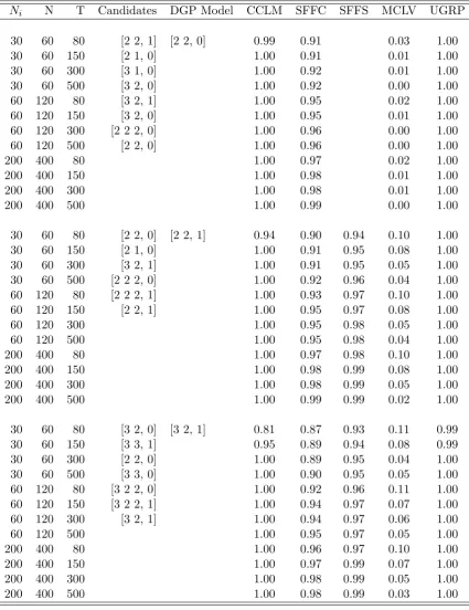
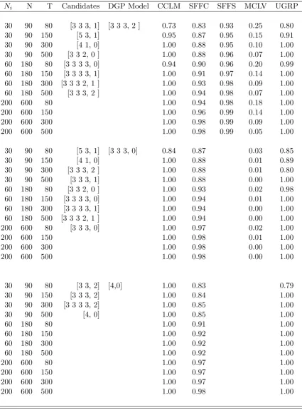
Ni N T Candidates DGP Model CCLM SFFC SFFS MCLV UGRP

30 60 80 [2 2, 1] [2 2, 0] 0.99 0.91 0.03 1.00 30 60 150 [2 1, 0] 1.00 0.91 0.01 1.00 30 60 300 [3 1, 0] 1.00 0.92 0.01 1.00 30 60 500 [3 2, 0] 1.00 0.92 0.00 1.00 60 120 80 [3 2, 1] 1.00 0.95 0.02 1.00 60 120 150 [3 2, 0] 1.00 0.95 0.01 1.00 60 120 300 [2 2 2, 0] 1.00 0.96 0.00 1.00 60 120 500 [2 2, 0] 1.00 0.96 0.00 1.00 200 400 80 1.00 0.97 0.02 1.00 200 400 150 1.00 0.98 0.01 1.00 200 400 300 1.00 0.98 0.01 1.00 200 400 500 1.00 0.99 0.00 1.00

30 60 80 [2 2, 0] [2 2, 1] 0.94 0.90 0.94 0.10 1.00 30 60 150 [2 1, 0] 1.00 0.91 0.95 0.08 1.00 30 60 300 [3 2, 1] 1.00 0.91 0.95 0.05 1.00 30 60 500 [2 2 2, 0] 1.00 0.92 0.96 0.04 1.00 60 120 80 [2 2 2, 1] 1.00 0.93 0.97 0.10 1.00 60 120 150 [2 2, 1] 1.00 0.95 0.97 0.08 1.00 60 120 300 1.00 0.95 0.98 0.05 1.00 60 120 500 1.00 0.95 0.98 0.04 1.00 200 400 80 1.00 0.97 0.98 0.10 1.00 200 400 150 1.00 0.98 0.99 0.08 1.00 200 400 300 1.00 0.98 0.99 0.05 1.00 200 400 500 1.00 0.99 0.99 0.02 1.00

30 60 80 [3 2, 0] [3 2, 1] 0.81 0.87 0.93 0.11 0.99 30 60 150 [3 3, 1] 0.95 0.89 0.94 0.08 0.99 30 60 300 [2 2, 0] 1.00 0.89 0.95 0.04 1.00 30 60 500 [3 3, 0] 1.00 0.90 0.95 0.05 1.00 60 120 80 [3 2 2, 0] 1.00 0.92 0.96 0.11 1.00 60 120 150 [3 2 2, 1] 1.00 0.94 0.97 0.07 1.00 60 120 300 [3 2, 1] 1.00 0.94 0.97 0.06 1.00 60 120 500 1.00 0.95 0.97 0.05 1.00 200 400 80 1.00 0.96 0.97 0.10 1.00 200 400 150 1.00 0.97 0.99 0.07 1.00 200 400 300 1.00 0.98 0.99 0.05 1.00 200 400 500 1.00 0.98 0.99 0.03 1.00

Notes: Table 1-Table 5 report the results of estimation of a GFM in 1000 Monte Carlo simulation runs. Ni is the number of variables in a group. N is the total number of

variables in a model. T is the number of observations. In the column of Candidates we list all grouped factor models under consideration. CCLM is the proportion of correctly identified models. SF F C and SF F S are the average goodness of fit of the estimated common factors and group-specific factors to the true factors respectively. M CLV gives the average proportion of misclassified variables in all variables over 1000 runs. U GRP

Table 2: Estimation of grouped factor models

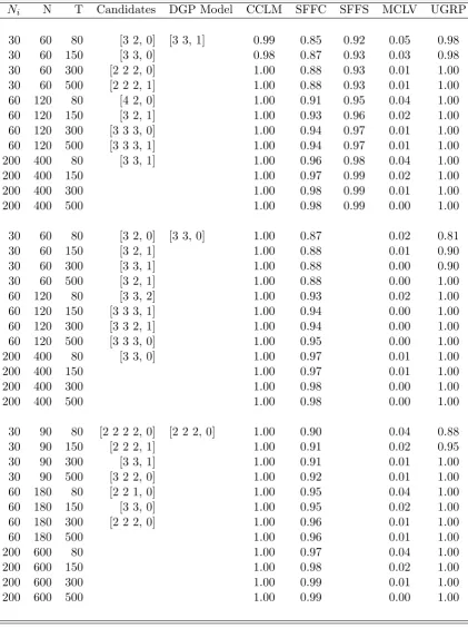
Ni N T Candidates DGP Model CCLM SFFC SFFS MCLV UGRP

30 60 80 [3 2, 0] [3 3, 1] 0.99 0.85 0.92 0.05 0.98 30 60 150 [3 3, 0] 0.98 0.87 0.93 0.03 0.98 30 60 300 [2 2 2, 0] 1.00 0.88 0.93 0.01 1.00 30 60 500 [2 2 2, 1] 1.00 0.88 0.93 0.01 1.00 60 120 80 [4 2, 0] 1.00 0.91 0.95 0.04 1.00 60 120 150 [3 2, 1] 1.00 0.93 0.96 0.02 1.00 60 120 300 [3 3 3, 0] 1.00 0.94 0.97 0.01 1.00 60 120 500 [3 3 3, 1] 1.00 0.94 0.97 0.01 1.00 200 400 80 [3 3, 1] 1.00 0.96 0.98 0.04 1.00 200 400 150 1.00 0.97 0.99 0.02 1.00 200 400 300 1.00 0.98 0.99 0.01 1.00 200 400 500 1.00 0.98 0.99 0.00 1.00

30 60 80 [3 2, 0] [3 3, 0] 1.00 0.87 0.02 0.81 30 60 150 [3 2, 1] 1.00 0.88 0.01 0.90 30 60 300 [3 3, 1] 1.00 0.88 0.00 0.90 30 60 500 [3 2, 1] 1.00 0.88 0.00 1.00 60 120 80 [3 3, 2] 1.00 0.93 0.02 1.00 60 120 150 [3 3 3, 1] 1.00 0.94 0.00 1.00 60 120 300 [3 3 2, 1] 1.00 0.94 0.00 1.00 60 120 500 [3 3 3, 0] 1.00 0.95 0.00 1.00 200 400 80 [3 3, 0] 1.00 0.97 0.01 1.00 200 400 150 1.00 0.97 0.01 1.00 200 400 300 1.00 0.98 0.00 1.00 200 400 500 1.00 0.98 0.00 1.00

Table 3: Estimation of grouped factor models

Ni N T Candidates DGP Model CCLM SFFC SFFS MCLV UGRP

30 90 80 [2 2 2 2, 0] [2 2 2, 1 ] 0.93 0.89 0.96 0.16 0.98 30 90 150 [3 2 2, 1] 0.99 0.91 0.96 0.11 1.00 30 90 300 [3 3, 1] 1.00 0.90 0.97 0.07 1.00 30 90 500 [3 2 2, 0] 1.00 0.92 0.97 0.06 1.00 60 180 80 [2 2 1, 0] 1.00 0.93 0.97 0.15 1.00 60 180 150 [3 3, 0] 1.00 0.95 0.98 0.10 1.00 60 180 300 [2 2 2, 1 ] 1.00 0.96 0.98 0.07 1.00 60 180 500 1.00 0.96 0.98 0.06 1.00 200 600 80 1.00 0.96 0.98 0.14 1.00 200 600 150 1.00 0.98 0.99 0.11 1.00 200 600 300 1.00 0.98 0.99 0.08 1.00 200 600 500 1.00 0.99 0.99 0.04 1.00

30 90 80 [3 3 2, 1] [3 2 2, 1] 0.72 0.87 0.95 0.18 0.72 30 90 150 [4 4, 1] 0.98 0.89 0.96 0.11 0.87 30 90 300 [4 3, 1] 1.00 0.90 0.96 0.08 0.92 30 90 500 [3 2 2 2, 1] 1.00 0.91 0.96 0.06 0.96 60 180 80 [3 2 2, 0] 0.95 0.93 0.97 0.15 0.99 60 180 150 [3 2 2, 1] 1.00 0.94 0.98 0.11 1.00 60 180 300 1.00 0.95 0.98 0.08 1.00 60 180 500 1.00 0.95 0.98 0.06 1.00 200 600 80 1.00 0.96 0.98 0.14 1.00 200 600 150 1.00 0.97 0.99 0.11 1.00 200 600 300 1.00 0.98 0.99 0.07 1.00 200 600 500 1.00 0.98 0.99 0.04 1.00

Table 4: Estimation of grouped factor models

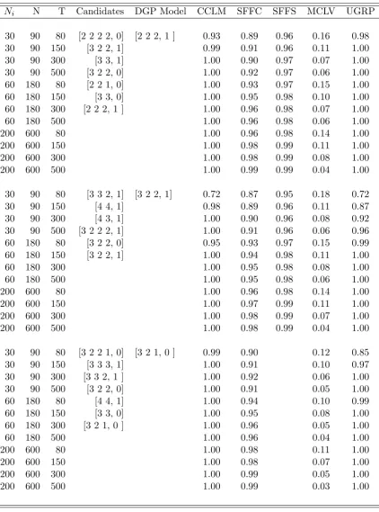
Ni N T Candidates DGP Model CCLM SFFC SFFS MCLV UGRP

30 90 80 [3 2 2 2, 0] [3 2 2, 0] 0.99 0.89 0.05 0.97 30 90 150 [3 3 3, 1] 0.99 0.90 0.03 1.00 30 90 300 [3 3 2, 1 ] 1.00 0.90 0.02 1.00 30 90 500 [3 2, 0] 1.00 0.91 0.01 0.90 60 180 80 [3 2 1, 0] 1.00 0.94 0.05 1.00 60 180 150 [4 3, 1] 1.00 0.95 0.02 1.00 60 180 300 [4 3, 0] 1.00 0.95 0.01 1.00 60 180 500 [3 2 2, 0] 1.00 0.95 0.01 1.00 200 600 80 1.00 0.97 0.04 1.00 200 600 150 1.00 0.98 0.02 1.00 200 600 300 1.00 0.98 0.01 1.00 200 600 500 1.00 0.99 0.00 1.00

30 90 80 [3 2 2 2, 0] [3 3 2, 1 ] 0.73 0.87 0.95 0.12 0.61 30 90 150 [3 3 3, 1] 0.93 0.88 0.96 0.08 0.81 30 90 300 [3 2 2, 1 ] 1.00 0.89 0.96 0.06 0.84 30 90 500 [3 3 1, 0] 1.00 0.89 0.96 0.04 0.94 60 180 80 [4 3, 0] 0.96 0.92 0.97 0.12 0.90 60 180 150 [4 3, 1] 1.00 0.94 0.97 0.08 1.00 60 180 300 [3 2 2, 0 ] 1.00 0.94 0.98 0.05 1.00 60 180 500 [3 3 2, 1 ] 1.00 0.95 0.98 0.05 1.00 200 600 80 0.99 0.96 0.98 0.11 1.00 200 600 150 1.00 0.97 0.99 0.08 1.00 200 600 300 1.00 0.98 0.99 0.05 1.00 200 600 500 1.00 0.98 0.99 0.02 1.00

Table 5: Estimation of grouped factor models

Ni N T Candidates DGP Model CCLM SFFC SFFS MCLV UGRP

30 90 80 [3 3 3, 1] [3 3 3, 2 ] 0.73 0.83 0.93 0.25 0.80 30 90 150 [5 3, 1] 0.95 0.87 0.95 0.15 0.91 30 90 300 [4 1, 0] 1.00 0.88 0.95 0.10 1.00 30 90 500 [3 3 2, 0 ] 1.00 0.88 0.96 0.07 1.00 60 180 80 [3 3 3 3, 0] 0.94 0.90 0.96 0.20 0.99 60 180 150 [3 3 3 3, 1] 1.00 0.91 0.97 0.14 1.00 60 180 300 [3 3 3 2, 1 ] 1.00 0.93 0.98 0.09 1.00 60 180 500 [3 3 3, 2 ] 1.00 0.94 0.98 0.07 1.00 200 600 80 1.00 0.94 0.98 0.18 1.00 200 600 150 1.00 0.96 0.99 0.14 1.00 200 600 300 1.00 0.98 0.99 0.09 1.00 200 600 500 1.00 0.98 0.99 0.05 1.00

30 90 80 [5 3, 1] [3 3 3, 0] 0.84 0.87 0.03 0.85 30 90 150 [4 1, 0] 1.00 0.88 0.01 0.89 30 90 300 [3 3 3, 2 ] 1.00 0.88 0.01 0.80 30 90 500 [3 3 3, 1] 1.00 0.88 0.00 1.00 60 180 80 [3 3 2, 0 ] 1.00 0.93 0.02 0.98 60 180 150 [3 3 3 3, 0] 1.00 0.94 0.01 1.00 60 180 300 [3 3 3 3, 1] 1.00 0.94 0.00 1.00 60 180 500 [3 3 3 2, 1 ] 1.00 0.94 0.00 1.00 200 600 80 [3 3 3, 0] 1.00 0.97 0.02 1.00 200 600 150 1.00 0.98 0.01 1.00 200 600 300 1.00 0.98 0.00 1.00 200 600 500 1.00 0.98 0.00 1.00

4.2

A Demonstrative Empirical Example

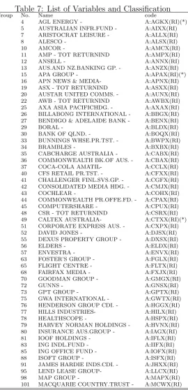
In this subsection we apply the grouped factor models with common and group-specific factors to stock returns in the Australian Stock Exchange. The data used in this exercise are stock returns of companies included in ASX200. ASX200 is one of the most important share index in Australia Stock Exchange. It accounts for about 85% of the market capitalization of all stocks listed in Australia Stock Exchange. The data set consists of monthly returns of shares included in ASX200 from 2004 to 2009. All together there are 168 variables and each of them contains 77 observations10_{. A full name list of the shares is given in Table 7 in the appendix.}

We transform the data so that each series has mean zero. Using theP C1p criterion

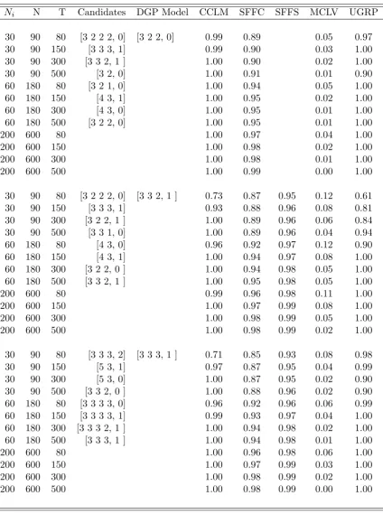
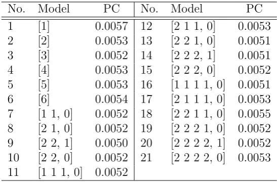
of Bai and Ng (2002) we identify that the dimension of the overall pervasive factor space is 3. After choosing K = 3 we investigate 15 potential candidate models. These 15 candidate models include all possible group configurations up to 4 groups within a three dimensional overall pervasive factor space. We decide not to include group configurations with more that 4 groups because in those cases it is highly probable that some group will contain less than 30 variables such that the model selection criterion would become very unreliable. The estimation results for the considered models are summarizes in Table 6.

Table 6: Estimation of Grouped Dynamic Factor Models for ASX200

No. Model PC No. Model PC

1 [1] 0.0057 12 [2 1 1, 0] 0.0053 2 [2] 0.0053 13 [2 2 1, 0] 0.0051 3 [3] 0.0052 14 [2 2 2, 1] 0.0051 4 [4] 0.0053 15 [2 2 2, 0] 0.0052 5 [5] 0.0053 16 [1 1 1 1, 0] 0.0051 6 [6] 0.0054 17 [2 1 1 1, 0] 0.0053 7 [1 1, 0] 0.0052 18 [2 2 1 1, 0] 0.0055 8 [2 1, 0] 0.0052 19 [2 2 2 1, 0] 0.0052 9 [2 2, 1] 0.0050 20 [2 2 2 2, 1] 0.0052 10 [2 2, 0] 0.0052 21 [2 2 2 2, 0] 0.0053 11 [1 1 1, 0] 0.0052

Notes: The columns under the headerP C report the values of the model selection criterion for the corresponding models.

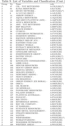
In Table 6 we see that [2 2, 1] obtains the lowest criterion value. We conclude, therefore, [2 2, 1] is the most suitable model for the data. The estimation procedure separated the 168 shares into two group (See Fig.2): the first group contains 115 shares and the second group contains 53 shares. Detailed information on grouping of the shares is given in Table 7. The grouping of shares depicts an industrial clustering in returns: the second group contains with few exceptions exclusively companies in resource sectors including mining, energy, and exploration, while the first group contains companies from other industries. Among the 53 companies in the smaller group there are only 6 companies (See (*) in Table 9.) that are not in the ming

10_{Due to missing data in the investigation periods we include only 168 shares in steady of 200}

Figure 1: ASX200 shares in two groups in the factor space

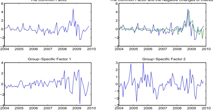
and energy sectors. The first group contains 115 companies, among which only 6 companies (See (*) in Table 8 and 9.) are in the mining and energy sectors. This industrial clustering allows us to interpret the estimation results in the following way: we call the second group the resource group and the first group the non-resource group. The common factor of the two groups drives shares in both groups. It reflects the overall economic and financial situation in Australia. The group-specific factor of the resource group can be called resource-factor. It reflects the special business conditions in the resource sector. The group-specific factor of the non-resource group drives the shares in the non-resource sectors. The estimated common factor and the group-specific factors of the two groups are given in Fig. 2. In the upper left penal we

2004 2005 2006 2007 2008 2009 2010 4

2 0 2 4 6

The!Common!Factor

2004 2005 2006 2007 2008 2009 2010 4

2 0 2 4 6

The!Common!Factor!and!the!Negative!Changes!of!Interest!Rate

2004 2005 2006 2007 2008 2009 2010 4

2 0 2 4

Group Specific!Factor!1

2004 2005 2006 2007 2008 2009 2010 3

2 1 0 1 2 3

Group Specific!Factor!2

Figure 2: Common Factors and Group-specific Factors