Munich Personal RePEc Archive
FDI and Local Financial Market
Development:A Granger Causality Test
Using Panel Data
Abdel Aal Mahmoud, Ashraf
George Washington University, university of Rome "Tor Vergata"
27 August 2010
Online at
https://mpra.ub.uni-muenchen.de/24654/
FOREIGN DIRECT INVESTMENT AND LOCAL FINANCIAL
MARKET DEVELOPMENT: A GRANGER
CAUSALITY TEST USING PANEL DATA
Ashraf Abdelaal Mahmoud1 University of Rome Torvergata Visiting researcher at School of Business
George Washington University
Abstract
This paper reports the findings of Granger causality tests on the relationship between foreign
direct investment (henceforth, FDI) and local financial market development across 62
countries from 1996 to 2007. In this paper we explore whether local financial market
development is important in catalyzing the flow of foreign direct investment. findings results
are robust to different measures of financial market development. Furthermore, the results
indicate that most of the causal links are found in Non OECD, Low income and Lower middle
Income countries.
Keywords : FDI; Financial market,Capital markets; Credit markets;
JEL classification F21;P45;O16;G1
1
Author Details: Ashraf Abd el aal Mahmoud, Junior Research at European research center – George Washington University, 2033 K street,NW Washington DC, 20009, United states. Tel: +2024362551 Email: [email protected] .
1.Introduction
The literature on FDI has advanced several explanations of those links between financial
market development and FDI inflows across a number of developing as well as developed
countries. Greenwood and Jovanovic (1990) and King and Levine (1993b) show that
financial market development reduces informational frictions and improves resource
allocation more efficiently. Hermes et al ( 2003) shows that FDI plays an important role in
contributing to economic growth but the level of financial development is crucial for these
positive effects to be realized. Alfaro et al. (2004) and Choong, et al.(2005) show that better
developed financial systems tend to benefit more from FDI. Omran, et al (2003) show that
domestic financial reforms should precede policies promoting FDI . Beck, et al. (2000)
suggest that financial systems are important for both productivity and development. Ashraf
Abdelaal (2010) show that Countries with better financial systems, and healthy business
environment are able to attract more FDI Rebecca M., et al (2009 ) examined the volatility
of capital flows (FDI, portfolio flows, and other debt flows) following the liberalization of
financial market and they found that capital flows are responding differently to financial
liberalization. Surprisingly, portfolio flows appear to show little response to capital
liberalization, while FDI flows show significant increases in volatility, particularly for the
emerging markets.
The empirical literature suggests that FDI inflows depend conditionally on host country
characteristics, De Mello (1999) and Zhang, K.H. (2001).
Table (1) FDI inflow
FDI inflow Value (billion dollars) % GDP
1986 1996 2006 1986 1996 2006
World 86 390 1461 0.6 1.3 3
Developed economies 71 237 973 0,6 1 2.7 Developing economies 16 147 434 0.6 2.3 3.6 Sub-Saharan Africa 2 0.7 3.7 38 0.4 1.9 7.6
COMESA 1 1 18 1 0.7 6.07
Source : UNCTAD(2009), World Investment Report .FDI inflow comprise capital provided (either directly or through other related enterprises) by a foreign direct investor to a FDI enterprise, or capital received by a foreign direct investor from a FDI enterprise. FDI includes the three following components: equity capital, reinvested earnings and intra-company loans. Equity capital is the foreign direct investor's purchase of shares of an enterprise in a country other than that of its residence. Reinvested earnings comprise the direct investor's share (in proportion to direct equity participation) of earnings not distributed as dividends by affiliates or earnings not remitted to the direct investor. Such retained profits by affiliates are reinvested. Intra-company loans or intra-company debt transactions refer to short- or long-term borrowing and lending of funds between direct investors (parent enterprises) and affiliate enterprises.
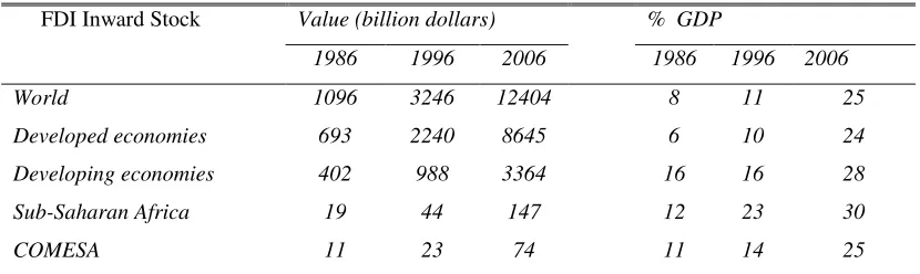
Table (2) FDI Inward Stock
FDI Inward Stock Value (billion dollars) % GDP
1986 1996 2006 1986 1996 2006
World 1096 3246 12404 8 11 25
Developed economies 693 2240 8645 6 10 24 Developing economies 402 988 3364 16 16 28 Sub-Saharan Africa 19 44 147 12 23 30
COMESA 11 23 74 11 14 25
Source :UNCTAD(2009), World Investment Report, FDI stock is the value of the share of their capital and reserves (including retained profits) attributable to the parent enterprise, plus the net indebtedness of affiliates to the parent enterprises
Flows of FDI have grown considerably in recent decades. In 1986, the level of FDI inflows stood at
US$ 86 Billion, and by 2006, it stood at US$ 1461 Billion. FDI flows have increased from
approximately 0.6% of world GDP at the beginning of the 1980s to a share between 2% and 3% since
the end of millennium (see Table 1).
FDI stocks have increased from a level of about 8% of world GDP at the beginning of the 1980s to
25% of world GDP in 2006 (see Table 2).FDI now represents the largest component of net resource
flows to developing countries, surpassing official development assistance (ODA), portfolio
investments, and bank loans Miyamoto( 2003).
2
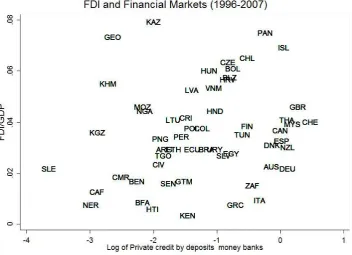
[image:4.595.89.507.87.212.2] [image:4.595.91.506.337.461.2]Source: Author elaboration (FDI/GDP source UNCTAD(2009), Privet credit by deposit source IMF’s International Financial Statistics, October 2008 )
[image:5.595.124.477.78.333.2]Fig. 1. Countries in this plot are the 64 countries (the sample data of this paper) .
Fig. 1. data on FDI and financial development shows the links between financial market development
(Private credit to deposits)3 and FDI inflows, which consider the motivation of this work i.e. countries
with better developed financial markets are able to absorb more from FDI to promote their economic
growth but the level of financial development is crucial for these positive effects to be realized.
In a trade, English capital is instantly at the disposal of persons capable of understanding the new
opportunities and making good use of them. In countries where there is little money to lend
enterprising traders are long kept back, because they cannot at once borrow the capital, without which
skill and knowledge are useless Bagehot ( 1873).
James Ang (2009) shows that efficient financial system facilitates FDI to create backward linkages,
which are beneficial to the local suppliers in the form of improved production efficiency. This implies
that financial market development plays a crucial role in the host country and its ability to attract FDI
and absorbs the benefits associated with it, Durham (2004) observed that the deeper financial systems
absorb capital inflows such as FDI.
3
Furthermore, financial markets affect both the financing of investment and day-to-day business
activities. Wurgler ( 2000) shows that even if financial development does not lead to higher levels of
investment, it seems to allocate the existing investment better.
In this paper, we examine whether better-developed financial markets are able to catalyze the flow of
foreign direct investment . To do this, we use a battery of financial market variables that exist in the
literature
The remainder of the paper is organized as follows: data are defined in Section 2; empirical results are
discussed in Section 3; and Section 4 concludes.
2.Data
This section describes the data used in the empirical analysis, specifically the measures of FDI, and
financial market development indicators , One of the fundamental problems inherent in literature is
that, to date, no specific causality analysis of the mutual relationship between FDI and Local financial
market development indicators has been conducted. The reason is that sufficiently long time series
necessary for using Granger causality tests are not available. However, recent theoretical
developments in Granger causality methods have made tests using relatively short time series possible
through the use of panel data approach4, adapting the methodology proposed by (Larrain et al., 1997;
Hurlin and Venet, 2001 Robert et al,2005) and recently applied by Erdil and Yetkiner (2008).
I test for Granger causality between two variables FDI and local financial market development
indicators : First, FDI, measured by the net inflow of foreign direct investment/GDP, FDI is defined as
the net inflows of investment to acquire a lasting management interest (10% or more of voting stock)
in an enterprise operating in an economy other than that of the investor. It is the sum of equity capital,
reinvestment of earnings, long-term capital and short-term capital as shown in the balance of
payments.FDI inflows with a negative sign indicate that at least one of the three components of FDI is
negative and not offset by positive amounts of the remaining components. These are called reverse
4
investment or disinvestment. The data are from United Nations Conference on Trade and
Development (UNCTAD) 2009 FDI database.
Second, local financial market development proxied by different measure which can be classified into
two levels :those relating to the banking sector and those relating to the equity markets.
For the first group, we will use first, Private Credit by Deposit Money Banks to GDP (henceforth,
PCDBGDP) and second, Private Credit by Deposit Money Banks and Other Financial
Institutions to GDP (henceforth, PCDBOGDP). They are the measures of the activity of financial
intermediaries in one of its main function: channeling savings to investors .Both indicators have been
used by researchers, the first by Levine and Zervos (1998), and the second by Levine, Loayza and Beck
(1999)and Beck, Levine, and Loayza (1999).
Third , liquid liabilities of the financial system (henceforth, LLGDP): equals currency plus demand
and interest-bearing liabilities of banks and other financial intermediaries divided by GDP. This is the
broadest available indicator of financial intermediation, since it includes all three financial sectors.
Liquid Liabilities is a typical measure of financial depth and thus of the overall size of the financial
sector, without distinguishing between the financial sectors or between the use of liabilities.
Fourth, Deposit Money Banks Assets to Total Financial Assets (henceforth, DBACBA): This
measure has been used as a measure of financial development by, among others, King and Levine
(1993a,b) and Levine, Loayza, and Beck (1998) and equals the ratio of deposit money banks assets and
the sum of deposit money and central bank assets.
For the second group, To measure the activity or liquidity of the stock markets we use stock market
total value traded to GDP(henceforth, SMTVT), which is defined as total shares traded on the stock
market exchange divided by GDP., and as indicator of the size of the stock market we use the stock
market capitalization to GDP ratio (henceforth, STMK)which equals the value of listed shares
divided by GDP.
Data for financial variables are available from the World Bank Financial Structure Database. Our
sample comprises 62 countries from 1996 to 2007.These countries were classified into three groups
low-income countries, the second consists of 50 middle-low-income countries and the third consists of 25
high-income countries
3. Empirical analysis
Consider a time-stationary VAR representation, adapted to a panel data context. For each individual I
have :
With and and where and are i.i.d (0 , ) ,
i.i.d ( 0 , ), respectively.
First step : The hypotheses to be tested are the homogenous non-causality hypotheses, given
by:
In the general case, the test statistics can be computed by the following Wald test proposed by
Hurlin and Venet (2001)
where SN denotes the total number of observations, stands for the restricted sum of
squared residuals obtained under , whereas is unrestricted sum of squared residual
computed from equations 4 and 5. This procedure also follows a standard Granger causality
assumption where the variables entered into the system need to be time-stationary. Thus, the
two variables are subjected to Levin, Lin and Chu (2002) and Im, Pesaran and Shin (IPS) Test For equation (1)
(1997) which are the most widely used methods for panel data unit root tests in the literature.
the null hypothesis is that there is unit root. unit root testing.
Table 3 Combined results of the panel unit root tests for FDI and Financial market indicators in their levels using Levin, Lin and Chu (2002)
Country / Variable FDI/GDP Financial Market Indicators
PCDBGDP PCDBOGDP LLGDP DBACBA SMTVT STMK
All country -4.918*** -3.025** -4.254*** -7.619*** -6.778*** --- -4.62***
OECD -1.489† -5.712*** -5.694*** -4.576*** -3.769*** -0.200 -5.92***
Non OECD -5.882*** -0.721 -2.023*** 2.612 -5.799*** --- ---
Low Income -5.486*** 0.439 0.455 -0.857 0.820 --- ---
Lower Middle Income -3.224*** -2.220* -3.490*** -5.646*** -1.712* -0.196 --- Upper Middle Income -1.920* -0.422 -0.865 -6.229*** -19.66*** --- ---
[image:9.595.66.528.151.250.2]† if p < 0.10, * if p < 0.05; ** if p < 0.01; *** if p < 0.001
Table 4 Combined results of the panel unit root tests for FDI and Financial market indicators in their First difference using Levin, Lin and Chu (2002)
Country / Variable FDI/GDP Financial Market Indicators
PCDBGDP PCDBOGDP LLGDP DBACBA SMTVT STMK
All country -10.337*** -10.735*** -10.506*** -16.155*** -26.28*** --- -13.04***
OECD -3.224*** -11.028*** -10.291*** -6.166*** 2.43 -3.372*** -13.54***
Non OECD -11.302*** -11.273*** -8.979*** -15.007*** -26.60*** --- --- Low Income -8.125*** -5.297*** -4.773*** -6.713*** -6.490*** --- --- Lower Middle Income -5.986*** -3.202*** -4.134*** -16.757*** -37.03*** -2.996** --- Upper Middle Income -7.273*** -8.560*** -7.172*** -7.089*** -3.824*** --- ---
[image:9.595.52.542.296.393.2]† if p < 0.10, * if p < 0.05; ** if p < 0.01; *** if p < 0.001
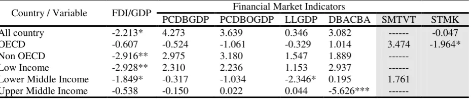
Table 5 Combined results of the panel unit root tests for FDI and Financial market indicators in their levels using Im, Pesaran and Shin (IPS) (1997)
Country / Variable FDI/GDP Financial Market Indicators
PCDBGDP PCDBOGDP LLGDP DBACBA SMTVT STMK
All country -2.213* 4.273 3.639 0.346 3.082 --- -0.047
OECD -0.607 -0.524 -1.061 -0.329 1.014 3.474 -1.964*
Non OECD -2.916** 2.975 3.180 1.547 1.889 ---
Low Income -2.928** 2.310 2.236 1.153 2.937 ---
Lower Middle Income -1.849* -0.317 -1.034 -2.346* 0.195 1.761 Upper Middle Income -0.538 -0.150 0.022 0.044 -5.626*** ---
† if p < 0.10, * if p < 0.05; ** if p < 0.01; *** if p < 0.001
Table 6 Combined results of the panel unit root tests for FDI and Financial market indicators in their First difference using Im, Pesaran and Shin (IPS) (1997)
Country / Variable FDI/GDP Financial Market Indicators
PCDBGDP PCDBOGDP LLGDP DBACBA SMTVT STMK
All country -8.068*** -4.929*** -4.904*** -6.032*** -6.912*** --- -5.703***
OECD -2.710** -6.557*** -5.945*** -3.428*** 2.388 -1.800* -6.075***
Non OECD -8.711*** -5.540*** -4.465*** -5.755*** -6.850*** --- --- Low Income -6.231*** -2.454** -2.418** -2.127* -3.105** --- --- Lower Middle Income -4.646*** -2.115* -2.748** -5.191*** -9.490*** -1.301† --- Upper Middle Income -4.890*** -4.358*** -3.392*** -3.323*** -1.481† --- ---
† if p < 0.10, * if p < 0.05; ** if p < 0.01; *** if p < 0.001
Given these results, I ought to use stationary first difference level variables for conducting the
[image:9.595.70.535.453.551.2]investigation. I computed the panel data VAR (equation 1,2) with the usual FE estimator, the Fhnc
statistics are reported in Table 7and Table 8..
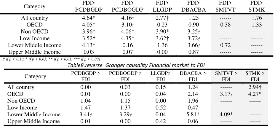
Table7. Granger causality analysis FDI to Financial market
Category FDI>
PCDBGDP
FDI> PCDBOGDP
FDI> LLGDP
FDI> DBACBA
FDI> SMTVT
FDI> STMK
All country 4.64* 4.16* 2.77† 1.25 --- 1.76
OECD 4.05* 3.10† 0.23 0.90 0.38 1.33
Non OECD 3.96* 4.06* 3.90* 3.25† --- ---
Low Income 3.52† 4.35* 3.62† 3.72† --- ---
Lower Middle Income 4.13* 0.16 1.36 3.66† 0.72 ---
Upper Middle Income 0.03 0.07 0.00 0.87 --- ---
[image:10.595.68.532.137.351.2]† if p < 0.10, * if p < 0.05; ** if p < 0.01; *** if p < 0.001
Table8.reverse Granger causality Financial market to FDI
Category PCDBGDP > FDI PCDBOGDP > FDI LLGDP> FDI DBACBA > FDI SMTVT > FDI STMK > FDI
All country 0.00 0.03 0.15 1.24 --- 2.94†
OECD 0.01 0.00 0.04 2.14 3.17† 4.27*
Non OECD 1.04 1.15 0.00 1.96 --- ---
Low Income 1.47 1.37 0.52 0.47 --- ---
Lower Middle Income 3.41† 3.29† 0.04 5.81* 4.09* ---
Upper Middle Income 0.01 0.00 0.42 0.06 --- ---
† if p < 0.10, * if p < 0.05; ** if p < 0.01; *** if p < 0.001
To investigate the contemporaneous relationships between FDI and Financial market
development indicators, we fitted the conventional panel data models. First, For all countries ,
FDI = f (Fin), We selected the estimator fixed or random effects using two diagnostic
statistics: Hausman (H) test statistics and Lagrange Multiplier (LM),The results are given in
Table 9.
The results are given in Table 8 and 9 Collectively, all models revealed a reasonable overall
fit. The interpretation is based on the latter specified models. For the All Countries, OECD
Countries ,Non OECD Countries, low income countries, and Lower Middle Income there are
a positive significant coefficient of banking sector indicators . Implies that countries with
high levels of financial market development attract more FDI.
For OECD and lower middle income countries, a positive significant coefficient of FDI is
Table(8) Contemporaneous relationships between FDI and Financial market Indicators
Category
FDI>PCDBGDP FDI>PCDBOGDP FDI>LLGDP FDI>DBACBA
Diagnostic
tests Cons Coef R
2 Diagnostic
tests Cons Coef R
2 Diagnostic
tests Cons Coef R
2 Diagnostic
tests Cons Coef R
2
All Countries
H: 131.25*** 0.370 9.62*** W: 0.65 H: 99.91*** 0.354 8.78*** W: 0.72 H: 49.29*** 0.191 4.66*** W: 0.64 H: 159.60*** 0.080 1.95† W: 0.66 LM: 0.84 0.0123 5.73*** B : 0.86 LM: 0.20 0.0128 5.35*** B : 0.95 LM: 0.62 0.011 6.70*** B : 0.83 LM: 5.56* 0.011 6.45*** B : 0.87
O: 0.76 O: 0.91 O: 0.83 O: 0.86
OECD Countries
H: 20.88*** 0.318 3.75*** W: 0.74 H: 16.22*** 0.297 3.31** W: 0.65 H: 7.29* 0.149 1.66† W: 0.02 H: 9.92** 0.493 1.93† W: 0.73 LM: 0.00 0.038 4.47*** B : 0.96 LM: 0.07 0.039 4.04*** B : 0.88 LM: 0.77 0.022 4.15*** B : 0.86 LM: 0.33 0.004 2.25* B : 0.83
O: 0.94 O: 0.76 O: 0.83 O: 0.83
Non OECD Countries
H: 92.03*** 0.424 10.44*** W: 0.76 H: 80.02*** 0.427 10.38*** W: 0.87 H: 30.98*** 0.228 5.04*** W: 0.60 H: 119.58*** 0.0705 1.69† W: 0.66 LM: 1.58 0.005 3.24** B : 0.95 LM: 0.92 0.005 3.24** B : 0.95 LM: 0.88 0.008 5.15*** B : 0.77 LM: 2.83† 0.013 6.55*** B : 0.79
O: 0.88 O: 0.94 O: 0.77 O: 0.78
Low Income
H: 68.13*** 0.284 3.62*** W: 0.87 H: 65.50*** 0.280 3.63*** W: 0.75 H: 26.83*** 0.145 1.85† W: 0.73 H: 46.74*** 0.0118 2.17* W: 0.68 LM: 3.51† 0.005 4.47*** B : 0.89 LM: 3.67† 0.005 4.15*** B : 0.96 LM: 0.03 0.009 3.59*** B : 0.94 LM: 0.38 0.0233 5.88*** B : 0.88
O: 0.85 O: 0.96 O: 0.94 O: 0.87
Lower Middle Income
H: 35.42*** 0.432 6.13*** W: 0.77 H: 30.91*** 0.426 5.98*** W: 0.77 H: 1.60 0.344 4.78*** W: 0.76 H: 228.76*** 0.164 2.15* W: 0.76 LM: 0.85 0. 0001 1.67† B : 0.95 LM: 0.57 0.005 2.16* B : 0.95 LM: 3.00† 0.003 1.69† B : 0.87 LM: 5.65* 0.008 3.09** B : 0.93
O: 0.88 O: 0.95 O: 0.86 O: 0.93
H = Hausman test : LM = Lagrange Multiplier : W = within : B= Between : O = Overall
† if p < 0.10, * if p < 0.05; ** if p < 0.01; *** if p < 0.001
Table(9) Contemporaneous relationships reverse causality between FDI and Financial market Indicators
Category
PCDBGDP >FDI PCDBOGDP >FDI DBACBA >FDI SMTVT > FDI
Diagnostic
tests Cons Coef R
2 Diagnostic
tests Cons Coef R
2 Diagnostic
tests Cons Coef R
2 Diagnostic
tests Cons Coef R
2
Lower Middle Income
H: 2.06 0.081 1.85† W: 0.09 H: 2.16 0.078 1.82† W: .093 H: 1.75 0.136 2.41* W: 0.11 H: 1.86 .018 1.78† W: 0.09 LM: 2.00 0.003 1.68† B : 0.01 LM: 1.91 0.003 1.70† B : 0.02 LM: 1.81 0.002 1.29 B : 0.01 LM: 3.08† 0.003 1.10 B : 0.31
O: 0.08 O: 0.08 O: 0.09 O: 0.08
H = Hausman test : LM = Lagrange Multiplier : W = within : B= Between : O = Overall
4.DISCUSSION
Our findings can be summarized in the following way. First for banking sector development indicators we
found that for all paper sample , financial market development levels Granger cause inward FDI flows ,and
by studying the reverse causality between Financial market development indicators and FDI inflow we
found no Granger causality relation except for lower Middle Income countries . The interpretations of this
result is that FDI goes to countries with good institutions and fundamentals, helping develop the domestic
financial system
Second, for liquidity of the stock markets indicators we found no Granger causality relation which Implies
that the liquidity of stock markets does not Granger cause inward FDI inflows That results are true for the
aggregate level data used in the current study for all countries . At the other extreme we found significant
direction of causality from FDI to liquidity of stock markets among lower middle income countries There
are two interpretations of this results First, FDI can be positively correlated with the number of firms in
capital markets, since foreign investors might want to finance part of their investment with external capital
or might want to recover their investment by selling equity in capital markets. Second, given that foreign
investors partly invest through purchasing existing equity, the liquidity of stock markets will likely rise.
Thus, the value traded domestically, the value traded internationally, or both might increase, depending on
where these purchases take place. In sum, FDI can Granger cause stock market development.
List Countries in the samples: Austria, Canada, Switzerland, Czech Republic Germany , Denmark, Spain ,
References
Ashraf Abdelaal Mahmoud (2010) ―FDI, local Financial Markets, employment and poverty alleviation‖ the
Seventh Annual JIBS/AIB Paper Development Workshop (PDW) in Rio de Janeiro, Brazil on Saturday, June 26, 2010
Alfaro, L. and A. Charlton (2007:20), ‗Growth and the Quality of Foreign Direct Investment: Is All FDI
Equal?‘, Harvard Business School Working Paper 07-072.
Alfaro L, Chanda A, Kalemli-Ozcan S, Sayek S (2004:372) FDI and economic growth: the role of local financial markets. Journal of international Economics 64:89–112
Bagehot, W. [1873] 1962 Lombard Street: a Description of the Money Market (with a New Introduction by Frank C. Genovese), Homewood, Ill. Richard Irwin.
Beck, T., Levine, R., and N. Loyaza (2000:1281) Finance and the Sources of Growth. Journal of Financial Economics 58, 261–300.
Carkovic, M., Levine, R., (2003:387). Does Foreign Direct Investment Accelerate Economic Growth? University of Minnesota, Working Paper.
Chuhan, Punam & Perez-Quiros, Gabriel & Popper, Helen, (1996:81). "International capital flows : do short-term investment and direct investment differ?," Policy Research Working Paper Series 1669, The World Bank
Chee-Keong Choong & Zulkornain Yusop & Siew-Choo Soo, (2005:5). "Foreign Direct Investment And Economic Growth In Malaysia: The Role Of Domestic Financial Sector," The Singapore Economic Review
(SER), World Scientific Publishing Co. Pte. Ltd., vol. 50(02), pages 245-268
De Mello, M. (1996:25) ―Foreign Direct Investment, International Knowledge Transfers and Endogenous
Growth: Time Series Evidence‖ Mimeo. Department of Economics, University of Kent, Kent.
De Mello L. R. (1999:393). Foreign direct investment-led growth: evidence from time series and panel data.,
Oxford Economic Papers, No. 51, pp. 133-151.
Dollar, David, and Aart Kraay (2001:2102). ‗Growth is Good for the Poor‘. Washington DC: World Bank, Development Research Group
Durham, J. B. (2004:122) Absorptive Capacity and the Effects of Foreign Direct Investment and Equity Foreign Portfolio Investment on Economic Growth. European Economic Review. 48, 285–306.
Erdil, E. and Yetkiner, I.H. (2008:1), ―The Granger-causality between health care expenditure and output: a
panel data approach‖, Applied Economics, first published on 23 June 2008.
Fisher, R.A., (1932: ). Statistical Methods for Research Workers, 4th Edition. Oliver & Boyd, Edinburgh.
Greenwood J, Jovanovic B (1990:1346) Financial development, growth, and the distribution of income.
Hermes, Niels and Lensink, Robert(2003:129) 'Foreign direct investment, financial development and economic growth', Journal of Development Studies,40:1,142 — 163
Hurlin C, Venet B. (2001:77). Granger causality tests in panel data models with fixed coefficients. Working Paper. EURIsCO, Universit´e Paris IX Dauphin.
James Ang,( 2009:6). "Financial development and the FDI-growth nexus: the Malaysian experience,"
Applied Economics, Taylor and Francis Journals, vol. 41(13), pages 1595-1601
King RG, Levine R (1993b:1153) Finance, entrepreneurship, and growth: theory and evidence. Journal of Monetary Economics. 32:513–542
Kyung So Im, M. Hashem Pesaran, Yongcheol Shin, Testing for Unit Roots in Heterogeneous Panels. Journal of Econometrics, 2003, 115, 53-74. Earlier version available as unpublished Working Paper, Dept. of Applied Economics, University of Cambridge, Dec 1997,
(http://www.econ.cam.ac.uk/faculty/pesaran/lm.pdf)
Miyamoto, K. (2003:48). Human capital formation and foreign direct investment in developing countries.
Technical Paper No. 211, OECD, Paris.
Omran M. & Bolbol A. (2003:10) . Foreign Direct Investment, Financial Development, and Economic Growth: Evidence from the Arab Countries Review of Middle East Economics and Finance, Vol. 1, No. 3, pp. 231-249
Rebecca M. Neumann, a, , Ron Penla and Altin Tankua (2009:7) . Volatility 27of capital flows and financial liberalization: Do specific flows respond differently? International Review of Economics & Finance Volume 18, Issue 3, June 2009, Pages 488-501
Robert Hoffmann & Chew-Ging Lee & Bala Ramasamy & Matthew Yeung, (2005:19). "FDI and pollution: a granger causality test using panel data," Journal of International Development, John Wiley & Sons, Ltd., vol. 17(3), pages 311-317.
Zhang, K.H. (2001:129), Does foreign direct investment promote economic growth? Evidence from East Asia and Latin America ,journal Contemporary Economic Policy, 19(2), 175-185