Optimization and Prediction Approaches for Flexible Routing in Dynamic Environment FMS

(1)

Optimization and Prediction Approaches for Flexible

Routing in Dynamic Environment FMS

Jaber Abu Qudeiri

1,*

_{, Usama Umer}

1

_{, Fayiz Abu Khadra}

2

_{, H.M.A. Hussein}

3

1_{Advanced Manufacturing Institute, King Saud University, Saudi Arabia} 2_{Faculty of Engineering, King Abdulaziz University, Saudi Arabia}

3_{Department of Mechanical Engineering, Faculty of Engineering, Helwan University, Egypt}

Abstract

Recently, many production systems that work in dynamic environment are widely used in high volume industries. Increasing the product varieties in dynamic environment Flexible Manufacturing Systems (FMS) have gained more importance due to growing production lines’ complexity. Increasing the customers demand to diversified products and rapid changing of the need to certain types of products require an FMS with high ability to adapt any change in production ratio during production. This paper introduces a Two Stages Approach (TSA) to increase the flexibility of the FMS to any change of the production ratios during production. The first stage of TSA is to propose a Genetic Algorithm (GA) based Production Simulator (GA-PS) to maximize the FMS throughput by optimizing the FLXible Routes (FLXR) for all products type at a given production ratio. The second stage is to propose a Neural Network (NN) approach to predict the routes of all products in FMS that can be used efficiently instead of a long, time-consuming GA-PS. TSA can improve the response of FMS to any change of the production ratio by finding a new FLXR that achieves the optimal throughput of the FMS within the new production ratios. Numerical examples will be applied to demonstrate applicability of the proposed approach. As a result, it could be ascertained that the proposed TSA is useful.

Keywords

FMS, Flexible Routing, Production Simulator, Genetic Algorithms, Neural Network

1. Introduction

Variety of products produce by Flexible Manufacturing Systems (FMS) have gained more and more importance because of growing production lines’ complexity and production costs and because an increasing demands for customized products. Conventionally, the product variety has been produced in a job shop or small batch operation. Job shop facilities are usually not suitable for large-volume mass production, because of low productivity and high production cost [1]. In contract, FMSs achieve high-volume mass

(2)

Notations

i index of part type, i=1, 2, …, l j operation index, j= 1, 2, …, O k machine index, k= 1, 2, …, M l No. of different part types

𝑀𝑀𝑖𝑖 Machine tool i

Oij operation j of part type i

𝑃𝑃𝑃𝑃𝑖𝑖𝑖𝑖𝑖𝑖 machining time of operation Oij in machine k

𝑆𝑆𝑃𝑃𝑖𝑖𝑖𝑖𝑖𝑖 setup time of operation Oij in machine k

𝑊𝑊𝑃𝑃𝑖𝑖𝑖𝑖𝑖𝑖 waiting time of the product i in front of the bay of machine k to perform operation Oij

𝑃𝑃𝑃𝑃𝑖𝑖𝑖𝑖 travel time of part time i through route Ri

𝑃𝑃𝑙𝑙𝑙𝑙𝑙𝑙𝑙𝑙\𝑢𝑢𝑢𝑢𝑙𝑙𝑙𝑙𝑙𝑙𝑙𝑙 time required to load\unload product TH throughput of the FMS

Ri route of part type i.

ni number of operations of product type i

𝑃𝑃𝑠𝑠 total time that product s spends to complete its tour through the FMS.

𝑂𝑂𝑝𝑝 No. of operations of part p.

𝑃𝑃𝑃𝑃0→1 time to move from load\unload station to machine of first operation

TTOs→0 time to move from last operation to load\unload station

TTa→b time to move from location a to location b F(i) fitness of individual number i

NI Number of individuals in each population

𝐼𝐼𝐼𝐼(𝑖𝑖 ) individual i

PR(i) selection probability of individual i

𝑃𝑃(𝑘𝑘) period between fitness F(k-1) and F(k)

𝑃𝑃𝑂𝑂𝑃𝑃(𝑘𝑘) population k

s Number of elitist individuals Cr Crossover rate

Mr Mutation rate

P number of parts to be produced

2. Modeling FMS and Model Assumptions

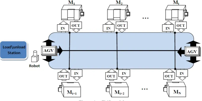
[image:2.595.133.475.564.735.2]

FMSis the major form of manufacturing system uses in high-volume mass production industries. FMS consider in this research consists of k different machine tools (CNC machining centers). Machine tools have finite local buffer capacity and uniform part delivery and holding pallets. All machine tools capable to process a required operation (Oij) on any part type, with different processing time (𝑃𝑃𝑃𝑃𝑖𝑖𝑖𝑖𝑖𝑖). In addition, the products inter and leave the FMS through load\unload station and handling system. The part travels between the FMS component by a number of automated guided vehicles (AGVs) with one pallet at a time. A typical structure of an FMS is shown in Figure 1. The FMS in this study is defined by a number of assumptions. These assumptions are summarized below.

(3)

FMS model assumptions

1. Large finite products variety can be produced by the FMS.

2. Handling of parts and materials in the FMS is done in single units (on unit-load pallets). 3. The products enter and leave the FMS through load\unload station

4. The time required to load and unload a part on\from the pallet is assumed to be 3 minutes. It needs one minute to move the ballet onto or from the AGV.

5. Each part is transferred on the unit-load pallet while in the system.

6. The layout of the FMS components is well defined, these components are fixed and the distance between each pair of them is known.

7. Buffer allocations are included in the system.

8. One operation can be performed in each machine tool of FMS at a time. 9. Tool change times are included in processing times.

10. All necessary components are available and fit in the system to execute any work order. 11. Processing time and setup time for each part type in each machine tool is known. 12. Some randomly selected machines can be considered as out of order.

13. Each machine is capable to perform different operations, but only one part can be processed at a time. 14. Once any operation is started it cannot be interrupted or divided.

15. Each machine tool stops N times an hour, and N<5. N is randomly selected. 16. Each machine tool stops for a quality check every P parts.

17. It takes one minutes to travel between two neighbors machine tools in vertical and horizontal directions.

3. Problem Definition

The FMS considered in this paper can produce l different part types; each type requires 𝑂𝑂𝑠𝑠 operations. Each operation can be processed by any machine tool (

M

_i

∈

M

) without any priority in machine tools. Parts can follow different routing among the machine tools to perform a job for P parts. The FMS scheduling problem is to find the optimal or near optimal route for each part type to maximize the throughput of the FMS. In this paper, GA is utilized to find efficient route that achieves the maximum throughout. The problem can be described mathematically as described below:

Given:

A set of machine tools M= {M1, M2, …, MK}, and a set of jobs J= {J1, J2, …, JK}, each job

i

J

,

∀

i

=

1 ,

2 ,

…

,

N

, consists of ni operations, each operation

O

_ij ,

∀

(

i

=

1 ,

2 ,

…

,

N

and j=1 ,2, …, ni)

can be processed in a machine tool Mi ,

M

_i

∈

M

and a production ratio for all product types : P1 : P2 :…: Pl

Determine: a route for each part type.

So that, TH (R1, R2, …, Rl) is maximum.

In order to find the number of part that can be produced by a given time, the total time, 𝑃𝑃𝑝𝑝, which the product type p spends during its trip through the FMS from the moment it leaves the load/unload station until it returns back to load/unload station is needed. The time required to produce

product of type p when it travels through route Rp can be calculated as follows:

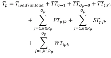
𝑃𝑃𝑝𝑝= 𝑃𝑃𝑙𝑙𝑙𝑙𝑙𝑙𝑙𝑙\𝑢𝑢𝑢𝑢𝑙𝑙𝑙𝑙𝑙𝑙𝑙𝑙+ 𝑃𝑃𝑃𝑃0→1+ 𝑃𝑃𝑃𝑃𝑂𝑂𝑝𝑝→0+ 𝑃𝑃𝑃𝑃(𝑖𝑖𝑖𝑖)

+ � 𝑃𝑃𝑃𝑃𝑝𝑝𝑖𝑖𝑖𝑖+ 𝑂𝑂𝑝𝑝

𝑖𝑖=1,𝑖𝑖∈𝑅𝑅𝑝𝑝

� 𝑆𝑆𝑃𝑃𝑝𝑝𝑖𝑖𝑖𝑖 𝑂𝑂𝑝𝑝

+ � 𝑊𝑊𝑃𝑃𝑖𝑖𝑝𝑝𝑖𝑖 𝑂𝑂𝑝𝑝

4. Genetic Algorithms for the FMS

Optimal Design

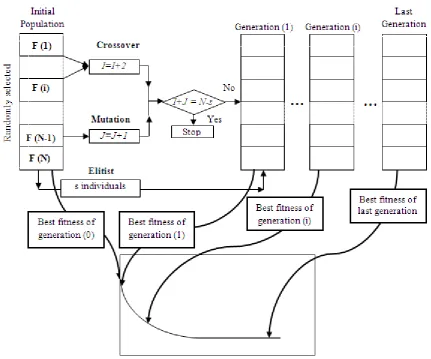
[image:3.595.335.525.376.475.2]

(4)

[image:4.595.89.521.74.433.2]

Figure 2 The GA outline 4.1. Matrix Encoding Method

The first step of GA is determination of the chromosome encoding method. The conventional linear genes encoding method is difficult to be used encode the complex arrangements of the route for all part products types. This is because there are many part types and each part type has different route. In this research, a Matrix Encoding Method (MEM) is proposed to express genes in individual. MEM encode the genes in chromosome as M × N matrix, where M is the number of the part types (part variety) and N is the number of operations required to produce each type. MEM expresses the individuals according to the number of part types and the number of operation required to produce each type. The individual using MEM is defined as follows.

𝐼𝐼𝑛𝑛𝑑𝑑𝑖𝑖𝑣𝑣𝑖𝑖𝑑𝑑𝑢𝑢𝑎𝑎𝑙𝑙 = ⎣ ⎢ ⎢ ⎢ ⎢ ⎢ ⎢ ⎢ ⎢ ⎡ l O l i l l j O j i j j O i O i

M

L

M

L

M

L

2 1 2 1 2 2 2 2 2 1 1 1 1 2 1 1 ⎦ ⎥ ⎥ ⎥ ⎥ ⎥ ⎥ ⎥ ⎥ ⎤ (1-a)

Where 𝑀𝑀_𝑖𝑖𝑖𝑖 is the machine that will operate operation i of the part type j, and l is number of part types and 𝑂𝑂𝑠𝑠 is number of operations required for part s. Equation (1-b) shows an example of the MEM encoding method













4 6 3 7 5 1 2 3 6 5 2 4 1 7 6 4 7 2 1 5 3

M

4

(1-b)

The expression matrix is not limited and it can be defined with any number of rows and columns, thus, any FMS structure and with any part varieties can be dealt with.

4.2. Initial Population and Selection of the Next Generations

(5)

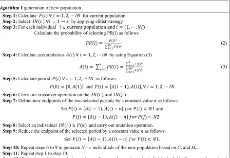
Algorithm 1 generation of new population

Step 1: Calculate 𝐹𝐹(𝑖𝑖) ∀ 𝑖𝑖 = 1, 2, ⋯ 𝐼𝐼𝐼𝐼 for current population

Step 2: Select 𝐼𝐼𝐼𝐼(𝑖𝑖 ) ∀𝑖𝑖 = 1 → 𝑠𝑠 by applying elitist strategy

Step 3: For each individual 𝑖𝑖 ∈ current population and 𝑖𝑖 = (1, ⋯ , 𝐼𝐼𝐼𝐼) Calculate the probability of selecting PR(i) as follows

𝑃𝑃𝑃𝑃(𝑖𝑖) = 𝐹𝐹(𝑖𝑖)2

�𝑁𝑁𝑁𝑁 𝐹𝐹(𝑖𝑖)2 𝑖𝑖=1

(2)

Step 4: Calculate accumulation 𝐴𝐴(𝑖𝑖) ∀ 𝑖𝑖 = 1, 2, ⋯ 𝐼𝐼𝐼𝐼 by using Equation (3)

𝐴𝐴(𝑖𝑖) = �𝑖𝑖_𝑖𝑖=1𝑃𝑃𝑃𝑃(𝑖𝑖)=�𝑖𝑖𝑖𝑖=1𝐹𝐹(𝑖𝑖)2

�𝑁𝑁𝑁𝑁 𝐹𝐹(𝑖𝑖)2

𝑖𝑖=1 (3) Step 5: Calculate period 𝑃𝑃(𝑖𝑖) ∀ 𝑖𝑖 = 1, 2, ⋯ 𝐼𝐼𝐼𝐼 as follows:

𝑃𝑃(0) = [0, 𝐴𝐴(1)] and 𝑃𝑃(𝑖𝑖) = [𝐴𝐴(𝑖𝑖 − 1), 𝐴𝐴(𝑖𝑖)], ∀ 𝑖𝑖 = 1, 2, ⋯ 𝐼𝐼𝐼𝐼

Step 6: Carry out crossover operation on the 𝐼𝐼𝐼𝐼(𝑖𝑖 ) and 𝐼𝐼𝐼𝐼(𝑗𝑗 )

Step 7: Define new endpoints of the two selected periods by a constant value n as follows:

Set 𝑃𝑃(𝑖𝑖) = [𝐴𝐴(𝑖𝑖 − 1), 𝐴𝐴(𝑖𝑖) − 𝑛𝑛] 𝑓𝑓𝑓𝑓𝑓𝑓 𝑃𝑃(𝑖𝑖) ⊂ 𝐼𝐼1 and 𝑃𝑃(𝑗𝑗) = [𝐴𝐴(𝑗𝑗 − 1), 𝐴𝐴(𝑗𝑗) − 𝑛𝑛] 𝑓𝑓𝑓𝑓𝑓𝑓 𝑃𝑃(𝑗𝑗) ⊂ 𝐼𝐼2

Step 8: Select an individual 𝐼𝐼𝐼𝐼(𝑖𝑖 ) ∈ 𝑃𝑃(𝑘𝑘) and carry out mutation operation.

Step 9: Reduce the endpoint of the selected period by a constant value n as follows:

Set 𝑃𝑃(𝑖𝑖) = [𝐴𝐴(𝑖𝑖 − 1), 𝐴𝐴(𝑖𝑖) − 𝑛𝑛] 𝑓𝑓𝑓𝑓𝑓𝑓 𝑃𝑃(𝑖𝑖) ⊂ 𝐼𝐼1.

Step 10: Repeat steps 6 to 9 to generate N – s individuals of the new population based on Cr and Mr.

Step 11: Repeat step 1 to step 10.

Step 12: Repeat step 11 to reach the optimum fitness value and set the individual of this fitness as the optimal

individual.

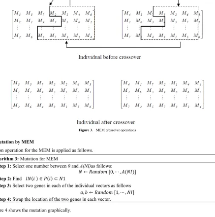
4.3. Crossover by MEM

MEM crossover is different from conventional crossover. MEM is applied using crossover line that passes through crossover points in the vectors, as shown in Figure 3. The MEM crossover is carried out using the following steps.

Algorithm 2: Crossover for MEM

Step 1: Select two numbers between 0 and A(NI)as follows:

𝐼𝐼1← 𝑃𝑃𝑎𝑎𝑛𝑛𝑑𝑑𝑓𝑓𝑅𝑅 [0, ⋯ , 𝐴𝐴(𝐼𝐼𝐼𝐼)] and 𝐼𝐼2← 𝑃𝑃𝑎𝑎𝑛𝑛𝑑𝑑𝑓𝑓𝑅𝑅 [0, ⋯ , 𝐴𝐴(𝐼𝐼𝐼𝐼)]

𝐼𝐼𝑓𝑓 𝐼𝐼1𝑎𝑎𝑛𝑛𝑑𝑑 𝐼𝐼2∈ 𝑃𝑃(𝑖𝑖), ∀𝑖𝑖 = 1, 2, ⋯ , 𝐼𝐼𝐼𝐼 𝑃𝑃ℎ𝑒𝑒𝑛𝑛, reselect 𝐼𝐼2

Step 2: Find 𝐼𝐼𝐼𝐼(𝑖𝑖 ) ∈ 𝑃𝑃(𝑖𝑖) ⊂ 𝐼𝐼1 𝑎𝑎𝑛𝑛𝑑𝑑 𝐼𝐼𝐼𝐼(𝑗𝑗 ) ∈ 𝑃𝑃(𝑗𝑗) ⊂ 𝐼𝐼2 , ∀ 𝑖𝑖, 𝑗𝑗 = 1, 2, ⋯ 𝐼𝐼𝐼𝐼

Step 3: Select l number of crossover points, CPi ,

∀

i

=

1,

2,

...,

l

as follows:

𝐶𝐶𝑃𝑃𝑖𝑖← 𝑃𝑃𝑎𝑎𝑛𝑛𝑑𝑑𝑓𝑓𝑅𝑅 [1, ⋯ , 𝑖𝑖, … , 𝑂𝑂 − 1]

[image:5.595.74.547.78.403.2]

Step 4: Exchange the genes after crossover line between the two individual.

(6)

[image:6.595.105.505.89.306.2]

Figure 3. MEM crossover operations

4.4. Mutation by MEM

Mutation operation for the MEM is applied as follows.

Algorithm 3: Mutation for MEM

Step 1: Select one number between 0 and A(NI)as follows:

𝐼𝐼 ← 𝑃𝑃𝑎𝑎𝑛𝑛𝑑𝑑𝑓𝑓𝑅𝑅 [0, ⋯ , 𝐴𝐴(𝐼𝐼𝐼𝐼)]

Step 2: Find 𝐼𝐼𝐼𝐼(𝑖𝑖 ) ∈ 𝑃𝑃(𝑖𝑖) ⊂ 𝐼𝐼1

Step 3: Select two genes in each of the individual vectors as follows

𝑎𝑎, 𝑏𝑏 ← 𝑃𝑃𝑎𝑎𝑛𝑛𝑑𝑑𝑓𝑓𝑅𝑅 [1, ⋯ , 𝐼𝐼𝐼𝐼]

Step 4: Swap the location of the two genes in each vector.

Figure 4 shows the mutation graphically.

Figure 4. Swap mutation

5. GA based Production Simulator

[image:6.595.86.524.94.535.2]

(7)

Algorithm 4: PSS algorithm

Step 1: Generate randomly the initial population with N individuals.

Step 1: Generate POP(0) as follows:

Select 𝐼𝐼𝐼𝐼(𝑖𝑖 ) ← 𝑃𝑃𝑎𝑎𝑛𝑛𝑑𝑑𝑓𝑓𝑅𝑅

⎣ ⎢ ⎢ ⎢

⎡

M

₁1 ⋯

M

1_Os

⋮ ⋮ ⋮

p

M

₁ ⋯

M

_Osp _⎦⎥ ⎥ ⎥ ⎤

, ∀𝑖𝑖 = 1 → 𝐼𝐼𝐼𝐼

Step 2: Read all characteristics of the desired FMS.

Step 3: Calculate 𝐹𝐹(𝑖𝑖) ∀ 𝑖𝑖 = 1, 2, ⋯ 𝐼𝐼𝐼𝐼 for current population

Step 4: Select 𝐼𝐼𝐼𝐼(𝑖𝑖 ) ∀𝑖𝑖 = 1 → 𝑠𝑠 by applying elitist strategy.

Step 5: Calculate PRi, ∀i =1,2,...,NI

Step 6: Carry out GA operations.

Step 7: If (Cr × NI + Mr × NI) = NI – s, then, continue to step 8, if not, return to step 6.

Step 8: Regard the generated individuals as the next generation population.

[image:7.595.100.533.178.549.2]

Step 9: Repeat until fitness reaches its maximum value.

Figure 5. Production simulator system

6. Prediction the Flexible Routing

To reduce the computational time for the routes determination required by the GA-PS, NN is introduces. NN learns the relationships between input data and output data and generalizes those relationships to unseen data. In this stage the NN is trained and introduced to predict the routes of product produced by a certain FMS. The algorithm of this stage is carried out using the following steps.

Algorithm 5: NN procedure

Step1: Construct the NN structure

Step2: Train the NN with some the routes resulted by

GA-PS in the first stage.

Step3: Validate the NN by the rest of routes.

7. Case Studies

7.1. Simulation Example

To show efficacy of the proposed simulation and prediction models, a simulation has been performed. The simulation is run to produce a specific number of products. The FMS consists of

(8)

7.2. GA and NN Parameters

The following GA parameters are selected after run the simulation several trials:

Population size of 100, probability of crossover of 0.9 and probability of mutation of 0.05 are used. The simulation is run to 500 generations. To train the NN, the three layers: input, hidden and output are selected; the three layers are 24, 23, and 1 respectively.

7.3. Simulations Results

Based on the GA-PS results, the routes of all products type are optimized, the routes and the maximum fitness obtained from GA-PS and those predicted by NN are given in Tables 1.

8. Conclusions

In this paper, we presented TSA to increase the flexibility of the FMS to any change of the production ratios during production to find proper routes for all product types in FMS. TSA used PSS generated a set of routes groups. The generated routes groups were used to train ANN utilized GA-PS to find optimal Flexible routes for all products type at a given production ratio. Unique genetic operations were applied for efficient used of GA.

[image:8.595.59.552.324.396.2]

The GA-PS results were used to train the NN. The trained NN were then used instead of GA-PS to predict the routes of all product types. By this way, a long simulation time required by the simulation can be eliminated. Numerical simulation showed that the results of the simulation and the trained NN approach are closed to each other and prediction approach can be used efficiently instead of the simulation.

Table 1. Comparison fitness obtained from GA-PS and those predicted by NN

Production Ratio Number of Machines Routes Best Fitness

Acquired by PSS Predicted by ANN

1:2:4:5

8

Type 1 route: 2→5→4→5→3→2→1→2→5→3 Type 2 route: 4→8→8→7→7→2→3→7→1→8 Type 3 route: 6→3→4→1→7→8→3→3→4→7 Type 4 route: 4→5→6→3→7→8→7→8→6→6

10.978E003 11.1368E003

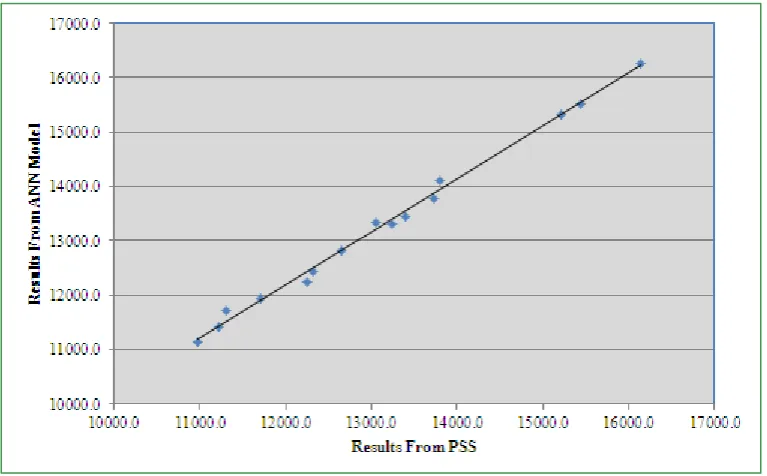
The regression analyses of outputs from the GA-PS and NN approach for the simulation is shown in Figure 6.

[image:8.595.114.498.420.658.2]

(9)

Acknowledgements

The authors would like to thank Fatima Alnijris Research Chair for Advanced Manufacturing Technology for the financial support provided for this research.

REFERENCES

[1] Groover, M. P. 1980. Automation, production systems, and computer-aided manufacturing. Englewood Cliffs, N.J.: Prentice-Hall.

[2] Mahdavi, I., A. H. F. M. Azar, and M. Bagherpour. 2009. Applying fuzzy rule based to flexible routing problem in a flexible manufacturing system. Paper read at Industrial Engineering and Engineering Management, 2009. IEEM 2009. IEEE International Conference on, 8-11 Dec. 2009. [3] Gershwin, S. B. 1994. Manufacturing systems engineering.

Englewood Cliffs, N.J.: PTR Prentice Hall.

[4] SabuncuoŸlu, I., and M. Lahmar. 2003. An Evaluative Study of Operation Grouping Policies in an FMS. International Journal of Flexible Manufacturing Systems 15 (3):217-239. [5] Shuiabi, E., V. Thomson, and N. Bhuiyan. 2005. Entropy as a

measure of operational flexibility. European Journal of Operational Research European Journal of Operational Research 165 (3):696-707.

[6] Bilkay, O., O. Anlagan, and S. E. Kilic. 2004. Job shop scheduling using fuzzy logic. The International Journal of Advanced Manufacturing Technology The International Journal of Advanced Manufacturing Technology 23 (7-8):606-619.

[7] Qudeiri, J. A., H. Yamamoto, and R. Ramli. 2009. Buffer size decision for Flexible Transfer Line with Rework Paths using Genetic Algorithm. IJISTA International Journal of Intelligent Systems Technologies and Applications 7 (2). [8] Ficko, M., M. Kovacic, and M. Brezocnik. 2004. Genetic

algorithms : a useful optimization method for manufacturing problems. Academic Journal of Manufacturing Engineering 2:21-26.

[9] Abu Qudeiri, J. Y. H. R. R. J. A. 2008. Genetic algorithm for buffer size and work station capacity in serial-parallel production lines. Artificial Life and Robotics 12 (1-2):1-2. [10]Goldberg, D. E. 1989. Genetic algorithms in search,

optimization, and machine learning. Reading, Mass.: Addison-Wesley Pub. Co.

[11]Altiok, T. 1997. Performance analysis of manufacturing systems. New York: Springer.

[12]Askin, R. G., and C. R. Standridge. 1993. Modeling and analysis of manufacturing systems. New York: Wiley. [13]Buzacott, J. A., and J. G. Shanthikumar. 1993. Stochastic

models of manufacturing systems. Englewood Cliffs, N.J.: Prentice Hall.

[14]Dallery, Y., and S. B. Gershwin. 1992. Manufacturing flow line systems: a review of models and analytical results. Queueing Syst Queueing Systems 12 (1-2):3-94.

[15]Heavey, C., H. T. Papadopoulos, and J. Browne. 1993. The throughput rate of multistation unreliable production lines. European Journal of Operational Research European Journal of Operational Research 68 (1):69-89.

[16]Helber, S. 1999. Performance Analysis of Flow Lines with Non-Linear Flow of Material. Lecture notes in economics and mathematical systems. (473):ALL.

[17]Papadopoulos, C. T., C. Heavey, and J. Browne. 1993. Queueing theory in manufacturing systems analysis and design. London; New York: Chapman & Hall.

[18]Papadopoulos, H. T., and C. Heavey. 1996. Queueing theory in manufacturing systems analysis and design: A classification of models for production and transfer lines. EOR</cja:jid> European Journal of Operational Research 92 (1):1-27.

[19]Perros, H. G. 1994. Queueing networks with blocking : exact and approximate solutions. New York: Oxford University Press.