Open Access
Research article
Choosing marginal or random-effects models for
longitudinal binary responses: application to self-reported disability
among older persons
Isabelle Carrière*
1
and Jean Bouyer
2
Address: 1INSERM Unité 500, 39 avenue Charles Flahault, 34093 MONTPELLIER, FRANCE and 2INSERM Unité 569-IFR69, 82 rue du Général Leclerc, 94276 LE KREMLIN BICETRE, FRANCE
Email: Isabelle Carrière* - [email protected]; Jean Bouyer - [email protected] * Corresponding author
Abstract
Background: Longitudinal studies with binary repeated outcomes are now widespread in epidemiology. The statistical analysis of these studies presents difficulties and standard methods are inadequate.
Methods: We consider strategies for modelling binary repeated responses and focus on two specific issues: the choice between marginal and random-effects models, and the choice of the time point origin. These issues are addressed using the example of self-reported disability in older women assessed annually for 6 years. The indicator of disability "needing help to go outdoors or home-confined" is used.
Results: In view of the observed associations between the responses for consecutive years, the baseline response was considered as a covariate. We compared the marginal and random-effects models first when only the influence of time and age is analysed and second when individual risk factors are studied in an aetiological perspective. There were substantial differences between the parameter estimates. They were due to differences between specific concepts related to the two models and the large between-individual heterogeneity revealed by the analysis.
Conclusions: A random-effects model appears to be most suitable for the analysis of self-reported disability in older women.
Background
In developed countries, disability in older persons is a ma-jor concern for public health authorities. Progress in med-ical care together with improved living conditions have led to longer life spans. One adverse consequence is that the number of very old people who are disabled is also in-creasing. The study of the succession of the different stages of disability, and of the ability to recover, together with the analysis of the risk factors for disability, are important issues for research in gerontology.
Longitudinal studies are more appropriate than cross-sec-tional studies which suffer various limitations due to bias-es such as the selective removal of disabled persons by institutionalisation, or differences in the proportions of disabled persons between age groups, also confounded with changes across generations [1]. Several authors [2] have analysed repeated measures of disability by compar-ing two by two time points. This method involves a very large number of tests and leads to partial results for fixed periods. The statistical analysis must take four main
char-Published: 5 December 2002
BMC Medical Research Methodology 2002, 2:15
Received: 29 July 2002 Accepted: 5 December 2002
This article is available from: http://www.biomedcentral.com/1471-2288/2/15
acteristics of the longitudinal data into account: 1) time may be an explanatory variable, 2) repeated observations for a subject are likely to be correlated, 3) the covariables may be time-dependent (they may vary through time for a subject), 4) missing data in the successive responses may induce a bias. Several statistical models developed for lon-gitudinal data have become more popular and there is software available for some of them. The problem of the choice of which to use remains.
Here, we present a strategy to model binary repeated re-sponses and to explain how to choose between marginal and random-effects models. The evolution of disability in older persons is used as an example to illustrate each step.
Methods
ExampleThe French EPIDOS study is a prospective multicentre study of the risk factors for hip fractures in 7575 women aged 75 years or older, included in 1992–1993 and re-cruited by mailing based on large population-based list-ings including electoral rolls [3]. Once in the study, these women were contacted by mail or telephone every four months to collect information about any falls and new fracture events. They had to complete a mail question-naire annually investigating hospitalisation, new health events, changes in weight, type of housing, ability to go outside, activities of daily life (ADL), instrumental activi-ties of daily life (IADL), medications used, and subjective health. This follow-up was initially planned for 4 years and then was extended to 6 years. In this paper we analyse the data from Montpellier (southern France), one of the 5 participating centres. We used the data from all the sub-jects included at this centre (1548 women) to analyse the evolution of disability.
The annual questionnaire was in some cases missing. This was mainly due to illness or to family events such as the death of the spouse. The women then postponed their an-swer.
Various indicators have been proposed to assess disability [4]. Needing help for going outdoors represents a first ev-ident level of functional limitation. It is easy to ev-identify and concerns both men and women. Therefore we chose "needing help to go outdoors or home-confined" as an in-dicator of disability. The annual response variable is bina-ry.
Marginal and random-effects models
In longitudinal studies, multiple assessments of the same subject at different time points are used and the within subject responses are then correlated. This correlation must be accounted for by analysis methods appropriate to the data [5]. Several models have been proposed for the
analysis of such data. Most of them are extensions of the well-known logistic regression that is a particular case of the generalized linear models with a logistic link function [6]. They are usually classified into marginal or random-effects models. Random-random-effects models are also called generalized linear mixed models or multilevel models or conditional models. However, this last term is ambiguous as several authors use it only for conditional maximum likelihood estimation [5] that we do not consider in this paper. Unlike linear models, the interpretation of the co-efficients of these two types of model differs (see below). The choice of one or the other depends on the objectives of the study.
Let Yij denote a binary outcome (in our example: needing help to go outdoors or home confined) corresponding to the jth response (jth year in the study in our example, j = 1 to ni) of the ith subject (i = 1 to K). Let also Xij be a de-sign matrix of covariates (1 × p vector, with first element being 1 for the intercept). The covariates may be fixed (for example age at baseline), or take different values at each year of the study (for example time or hospitalised for the last year). The marginal model, also called the popula-tion-averaged model [7], estimates the model thus:
logit (E (Yij | Xij)) = logit (P (Yij = 1 | Xij)) = Xij'β
whereas the random-effects model, also called the "sub-ject-specified models" [7], estimates the model as follows:
logit (P (Yij = 1 | Xij)) = Xij' βi
Thus, the marginal model supposes that the relationship between the outcome Y and the covariate X is the same for all the subjects, and the random-effects model allows this relationship to differ between subjects. To highlight this point, the random-effects model may also be written:
logit (E (Yij | Xij, Ui)) = X'ij (β* + Ui) = Xij' β* + Xij' Ui or:
logit (E (Yij | Xij, Zij, Ui)) = Xij' β* + Zij' Ui
where the random effects Ui are assumed to vary inde-pendently from one subject to another according to a common distribution. This distribution is often supposed to be normal with mean 0 and variance D. Zij is often a subvector of Xij, which means that random effects apply only to a part of the covariates and the intercept. The var-iance, D, has to be estimated and represents the extent of the unexplained between-individual variability.
equal. Hence, the estimators estimate different things[8] and the magnitude of the difference between β and β* is function of the variance, D [9].
Moreover, dependencies between observations over the time are handled differently in the two models. In the marginal model, it is popular to fit the vector of parame-ters, β, using the Generalized Estimating Equations (GEE) proposed by Liang and Zeger [10] wherein the covariance matrix is structured by using a working correlation matrix R(α) fully specified by the vector of parameters, α. This working correlation is assumed to be the same for all the subjects, reflecting an average dependence among the re-peated observations for all subjects. In contrast, the ran-dom-effects model allows this within-subjects dependency to vary from one subject to another, by the means of the random part of the covariable linear combi-nation. In the simplest case, only a random intercept is in-troduced
logit (E (Yij | Xij, Ui)) = Xij'β* + Ui0
Ui0 being an individual parameter of propensity to be-come disabled, constant through the time. For a given subject, whatever the interval of time between two re-sponses, the strength of dependency is then the same. If a random slope for the time covariable is added
logit (E (Yij | Xij, Ui)) = Xij' β* + Ui0 + Ui1 time
this individual strength of association increases or de-creases with the width of the interval.
In the marginal model, several specific choices of the structure of the working correlation matrix R(α) are pos-sible. For example, R(α) is called m-dependent if corr(Yij,Yik) = αt for t = 1, 2, ..., m and corr(Yij,Yik) = 0 for
t >m; R(α) is exchangeable if corr(Yij,Yik) = α for j ≠k, and it is unstructured if corr(Yij,Yik) = αik. An advantage of the marginal model, demonstrated by Liang and Zeger, is that
βand their robust variance are consistent (the estimator converges towards the parameter being estimated as the sample size increases) even when the correlation structure is misspecified. However, choosing the working correla-tion structure closest to the true structure increases the sta-tistical efficiency of the parameter estimator. Consequently, it is recommended to specify the working correlation as accurately as possible, based on the knowl-edge of the longitudinal process [11].
Concerning the estimating procedures, the GEE method for marginal models is not difficult to implement and is now available in the major statistical analysis packages. The procedures are more complex for the random-effects model. The most attractive of them directly maximizes an
approximate integrated likelihood. With non-linear mod-els computational-intensive integration methods, such as Gauss-Hermite quadrature, are necessary to evaluate the likelihood [12].
Different assumptions are required for the two models re-garding missing data. The marginal model using the GEE requires a missing data process completely at random (MCAR). Under this assumption, missingness does not depend on individual characteristics (observed or not). In contrast, random models only need the less stringent as-sumption of missing at random (MAR). In this process, the probability of missingness depends only on observed variables (previous covariates or outcomes) [13]. All mar-ginal models do not require the MCAR assumption. For example, Robins et all [14] proposed methods to allow for data that are MAR in marginal models, but these methods are more complicated to implement.
The interpretation of the coefficients βand β* also differs. Consider, for instance, the covariate X "living alone". The odds ratio OR* = exp(β*) represents the odds of the out-come (needing help to go outdoors or home confined) for a person living alone compared to the same person sup-posed not to live alone. It can be seen as an odds ratio ad-justed on unobserved individual characteristics. Under the marginal model, OR = exp(β) represents the averaged odds of the group living alone compared to the sub-group not living alone.
In the following sections we will first describe the data and then focus on the specific problems inherent to lon-gitudinal analyses: how to choose the time point origin and how to take into account the influence of time on re-sponses. Then, we will present an example of an estima-tion of risk factors including covariates fixed across time for a single subject, and time-dependent covariates.
Results
Description of the data
why we chose to perform a repeated measures analysis and not to use statistical methods analysing time before entering disability, such as Cox regression.
The study was initially planned to last 4 years, some wom-en refused to continue in years 5 and 6, and the number of those returning the completed questionnaire decreased most quickly between years 4 and 5 (Table 1). Some wom-en gave intermittwom-ent answers. For example, of the 970 women still providing a response in year 6, at least one observation in the previous years was missing for 150 (15 percent). The missingness partly depended on unob-served individual events (illness or family events) and is unlikely to be MCAR. The use of the marginal model is therefore questionable because an averaged effect is only poorly meaningful. The true time between yearly assess-ments and inclusion varied from one woman to another and the range tended to be higher at the end of the follow-up. Consequently, time is considered as a continuous co-variable. Vital status was known throughout the 6 years for all the participants, even those who no longer sent back the questionnaires. The total number of deaths was 294 (19 percent) by the end of the study.
Choice of the time point origin
The response Yi0 given by the ith subject at baseline may be handled in two ways. It can be considered either as a part of the longitudinal response, and thus the response vector has 7 elements corresponding to the times 0, 1, ..., 6 years, or as a baseline covariate, in which case the re-sponse vector has 6 elements. These two possibilities cor-respond to different structures for the raw data and are displayed in Tables 2 and 3. In the models studied (mar-ginal or random-effects model), the association between two successive responses is supposed to have the same structure through the whole survey. If the association be-tween baseline disability and the other responses differs from the association between the follow up responses, then it is better to consider the baseline response as a co-variable.
In our example, as in many cohort studies, the baseline ex-amination was exhaustive. The women were proposed
clinical and functional examinations (series of standard tests of physical performance) and a bone densitometry at the hospital. However, only those who felt well enough to undergo these tests were examined, probably introducing a selection bias at inclusion. During the follow-up, the women were only asked to complete a mailed question-naire that even physically dependent persons could an-swer. The profile of our sample changed through time, with the women becoming more and more physically de-pendent. At the beginning, many of the disabled women were probably only slightly disabled and thus there was the possibility of recovery. As time passed more women were severely disabled, and stayed so until the end of the study. Thus, the association between the responses for consecutive years is likely to be stronger in the last years. Also, the baseline response may be considered as a special case, less related to the following disabled states.
To check this, we examined the table of the odds ratios of being disabled for the year j (Yij) according to disability the previous years (Yi(j-t)). The association between two Table 1: Description of the data by year of assessment
Inclusion Year 1 Year 2 Year 3 Year 4 Year 5 Year 6
Total number of women with disability assessment 1548 1503 1450 1409 1294 1020 970
Percent of disabled women 29% 39% 41% 46% 47% 48% 52%
Time since inclusion (yrs)
Median 0.99 1.98 2.97 3.95 4.96 6.12
Range 0.91, 1.67 1.95, 2.44 2.93, 3.37 3.87, 4.53 4.87, 6.35 5.88, 6.94 Number of deaths for the preceding year 23 34 40 63 58 76
Table 2: Structure of the raw data when the baseline response is taken as a part of the reponse
Response Time Covariates l = 1, ... p
Time dependent covariates
l = 1, ....q
yi0 ti0 xi0l zi0l
yi1 ti1 xi0l zi1l
yi2 ti2 xi0l zi2l
yi3 ti3 xi0l zi3l
yi4 ti4 xi0l zi4l
yi5 ti5 xi0l zi5l
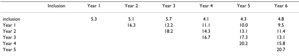
successive time points beyond baseline was stronger than that with the baseline response (Table 4). For instance, in the lower diagonal giving the association between two ob-servations separated by one year, the odds ratio between year 1 and the baseline is 5.3 whereas it is greater than 16 between year 2 and 1, and between the following pairs of years. In view of these results, the baseline response was considered as a covariate and the data were structured as shown in Table 3. There was also a tendency for correla-tions to decrease with increasing time differences (Table 4). For example, the odds ratio is 16.3 between year 1 and year 2 and 10.0 between year 1 and year 5. This observa-tion allows a better selecobserva-tion of the correlaobserva-tion structure, avoiding the use of an exchangeable working correlation matrix in marginal models, and introducing a random slope in random effect models.
Analysis of time and age evolution
The objective here is to evaluate the impact of time on the proportion of disabled women. We chose to use the age at entry (fixed covariable) and the time since baseline to characterize this phenomenon. Another solution would be to use the age at every response (as a time varying
cov-ariable) but our option allows the introduction of an in-teraction between the age at entry and the time since baseline to test whether the effect of time is more pro-nounced in the oldest women.
In view of the missingness process resulting in the sample differing at every assessment, and the possible selection bias at entry, the search for individual relationships using the random-effects model is more suitable than using population averaged associations. However the two mod-els are interesting to compare to show that the estimate parameters can be different, and to explain these differ-ences.
We used two methods to characterize the changes in disa-bility over time: the marginal model with the GEE ap-proach and the random model with likelihood integration. The random model had Gaussian random ef-fects and errors. We used the SAS procedures GENMOD with the REPEATED statement and an unstructured work-ing correlation matrix and also NLMIXED with the Gauss-Hermite quadrature integration method [12]. For the SAS code refer to Appendix (see Additional file 1). In the ran-Table 3: Structure of the raw data when the baseline response is taken as a baseline covariate
Response Time Response at t 0 Covariates l = 1, ... p Baseline values of the time dependent
cov-ariates l = 1, ....q
Time dependent cov-ariates l = 1, ....q
yi1 ti1 yi0 ...xi0l.... ...zi0l... ...zi1l...
yi2 ti2 yi0 ...xi0l.... ...zi0l... ...zi2l...
yi3 ti3 yi0 ...xi0l.... ...zi0l... ...zi3l...
yi4 ti4 yi0 ...xi0l.... ...zi0l... ...zi4l...
yi5 ti5 yi0 ...xi0l.... ...zi0l... ...zi5l...
yi6 ti6 yi0 ...xi0l... ...zi0l... ...zi6l...
Table 4: Odds ratios of being disabled at each year according to disability at the previous years
Inclusion Year 1 Year 2 Year 3 Year 4 Year 5 Year 6
inclusion 5.3 5.1 5.7 4.1 4.3 4.8
Year 1 16.3 12.2 11.1 10.0 9.5
Year 2 18.2 14.3 13.1 11.4
Year 3 16.7 17.3 13.1
Year 4 20.2 15.8
dom model, we determined the structure of the covari-ance introducing successively two random effects: random intercept and random slope for the time covari-ate.
In all the models, the following fixed effects were then tested: time since baseline (continuous variable), time square, age at entry (in years exceeding 74), interactions age × time and baseline inability to go outside without help. Only the time square effect was not significant, and was removed from the model. We also introduced an in-dicator variable for women dying within the 6-year peri-od. This is a simple way to take into account dropouts due to death, a difficulty often encountered in longitudinal studies in the elderly. The use of this time-fixed indicator was possible since information about death was known for the six years for all the women. The NLMIXED proce-dure converged and provided estimations only when the initial parameters were close to the final solution. We cal-culated successive models, beginning with a simple model with only a random intercept, and at each step we used the
previous estimate parameters as initialisation for the next estimation.
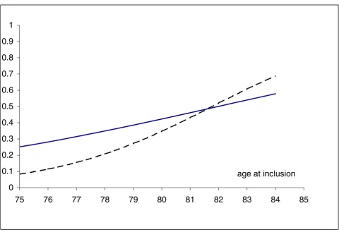
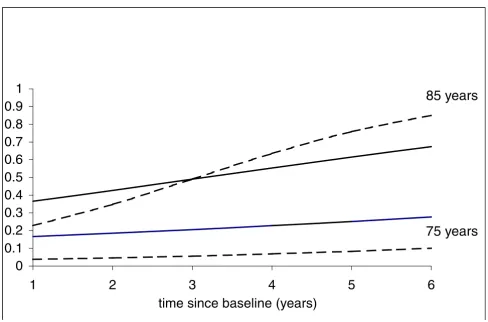
The results of the comparison between the 2 modelling strategies are shown in Table 5. The general conclusion is the same for the 2 models but the estimated parameters are different. For instance, the most important factor, baseline inability, is very significant in both, but parame-ter estimates differ from 1.54 to 3.18. The significant in-crease in risk of being disabled with age and time since baseline is illustrated in figure 1, presenting the averaged probability of disability, 5 years after the inclusion, in women able to go outside without help at baseline and who did not die during the study. In our cohort, recruited in 1992–1993, the probability of restricted mobility, 5 years later, was high, especially after the age of 80 years. Figure 2 shows the changes with time in two groups aged 75 and 85 years at entry. There was a significant interac-tion between age at entry and time, and consequently the risk of disability is accelerated in the oldest women.
Figure 1
Age at baseline and probability of disability at 5 years in women without disability at entry and surviving to the end of the study, GEE marginal model —, random model
---0
0.1
0.2
0.3
0.4
0.5
0.6
0.7
0.8
0.9
1
75
76
77
78
79
80
81
82
83
84
85
Differences between the estimators of the marginal and random-effects parameters are expected (see above). The marginal model expresses averaged relationships without taking into account the fact that the same subjects are con-sidered at each time point, whereas the random-effects model gives relationships conditionally on having certain
individual characteristics modelled by the random effects. In the case of only a random intercept, Nehaus et al [9] demonstrated that the estimates from the marginal model are systematically lower than those from the random model. This characteristic is shown in figures 1 and 2, where the curves from the marginal model are flatter than
Figure 2
Changes through time evolution of the probability of disability in women without disability at entry and surviving to the end of the study, aged 75 and 85 years at entry, GEE marginal model —, random model
---Table 5: Marginal model and random-effects models analysing the influence of time and age
Marginal model GEE Random model likelihood integration
Estimate SE p value Estimate SE p value
Intercept -1.83 0.12 < 0.0001 -3.61 0.25 < 0.0001
Time (years) 0.12 0.03 < 0.0001 0.17 0.06 0.002
Age at baseline* 0.09 0.02 < 0.0001 0.16 0.03 < 0.0001
Age* × time 0.01 0.004 0.003 0.04 0.009 < 0.0001
Baseline disability 1.54 0.10 < 0.0001 3.18 0.22 < 0.0001 Death during the study 0.68 0.12 < 0.0001 1.36 0.26 < 0.0001
Random intercept variance - - - 7.25 0.68 < 0.0001
Random slope variance - - - 0.18 0.04 < 0.0001
0
0.1
0.2
0.3
0.4
0.5
0.6
0.7
0.8
0.9
1
1
2
3
4
5
6
time since baseline (years)
the others. The differences between the estimates of the two approaches are largely dependent on the inter-indi-vidual heterogeneity. This heterogeneity can be assessed in the random models by looking at the intercept and slope variances.
In the random model, the random intercept variance is high. The estimate is 7.25, indicating that the variability of this individual additional intercept has a 95 percent width
of 10.6 ( × 1.96 × 2). If we consider the variability given by the fixed covariates (age varying from 75 to 85 years, baseline disability and death each varying from 0 to 1) the width is 6.14 (0.16 × 10 + 3.18 + 1.36). Hence the variability explained by these three fixed variables is lower than the unexplained between-individual variability. Sim-ilarly, the random slope variability has a 95 percent width of 1.66, whereas the variability explained by the age has a 95 percent width of 0.40 (0.04 × 10).
The probability of being disabled is therefore much more due to the woman's uncharacterised "frailty" than to age or to baseline disability. This wide between-individual heterogeneity explains the differences between the param-eter estimates of the marginal and random-effects models.
Analysis of risk factors
Changes with time expressed as age at entry and the time since baseline were modelled in the previous section. The
marginal and random-effects models can also be used to identify other risk factors for disability. It would also be interesting to test how the estimating algorithms behave when numerous covariables are jointly introduced.
We compared two multivariate models adjusted on the covariates presented in the previous section (age, time, in-teractions between age and time, baseline disability, still alive at the 6-year period) (see table 6). When numerous covariables are put in the model, the NLMIXED procedure may fail to integrate the likelihood or give non-stationary estimations. This non-optimal estimation can be diag-nosed by checking the gradient (vector of first derivative) of the negative log likelihood function for each parameter. These gradients are systematically provided by SAS in the results. If one of them is not close to zero, then the solu-tion cannot be considered to be valid. These problems of convergence were not encountered with the set of covari-ables shown in table 6. Two categories of covaricovari-ables were tested: variables collected at baseline (living at home alone, body mass index (BMI), visual acuity measured with Snellen letter test chart on a decimal scale, and per-ceived health) and variables that vary with time (hospital-ised at least once during last year, temporarily bed-confined during last year and number of falls during last year). Adjusted on all the others, all these factors were sig-nificant.
7 25.
Table 6: Marginal model and random-effects models analysing time-fixed and time varying covariates
Marginal model* GEE Random model* likelihood integration
Estimate SE p value Estimate SE p value
Baseline
Living alone -0.31 0.09 0.0004 -0.66 0.18 0.0002
BMI (kg/m2)
< 25 (ref) 0 0
25 – 29 0.30 0.10 0.002 0.69 0.20 0.0005
≥ 29 0.75 0.12 < 0.0001 1.46 0.23 < 0.0001
Visual acuity
≤ 2/10 0.64 0.20 0.001 1.21 0.35 0.0006
> 2/10 (ref) 0 0
Perceived health
Bad or very bad 0.76 0.15 < 0.0001 1.43 0.28 < 0.0001
Follow-up
Hospitalised (past year)
0.26 0.05 < 0.0001 0.49 0.11 < 0.0001
Temporarily bed confined (past year)
0.39 0.07 < 0.0001 0.73 0.15 < 0.0001
Number of falls ≥ 2 (past year)
0.23 0.08 0.004 0.49 0.15 0.0013
Discussion
We present the steps for choosing a model able to charac-terize disability taken as a binary response.
Several important points have to be considered in the analysis of repeated binary data. First, the choice between the marginal and random-effects models depends mainly on the aims of the study. If the goal is to predict a mean prevalence of disability over time in elderly people by sex or age group, the marginal model is suitable. In contrast, if the goal is to study the individual risk factors for aetio-logical considerations, the random-effects model is more suitable because it allows adjustment on non-observed in-dividual characteristics, and a better understanding of the underlying mechanism.
Second, the missing data process has to be examined. The marginal model using GEE assumes that the sample is rep-resentative of the whole population at each time point and the missing data is MCAR. This is unlikely to be the case in our example. The random-effects model assuming an MAR process is more appropriate. By the end of the study, half of the 37% of missing data were due to deaths and most were predictable from the previously collected data. The same probably applies to missing data due to chronic illnesses. Nevertheless, we cannot exclude the possibility that unobserved level of disability in our exam-ple may influence a part of the missing process. The mag-nitude of the potential bias introduced by non-random missingness should therefore be examined. A sensitivity analysis to assess the impact of missing data on subse-quent statistical inference would be worthwhile [15], but is beyond the scope of this paper.
Another important point is to determine whether the dis-ability indicator at baseline should be considered as a re-sponse or as a covariate. In epidemiological cohorts, the conditions in which responses are collected at baseline and during the follow-up are often different. The first re-sponse is often considered as a covariate but this choice has to be confirmed in view of the analysis of dependency between the responses.
The structure of the covariance between the repeated re-sponses has also to be chosen. In the marginal model, the inferences on the parameter estimates are asymptotically valid under any assumed structure but it is better to choose a structure corresponding to the data. In contrast, in the random model, the fixed and random parameters are simultaneously estimated and the choice of the covar-iance structure influences the final results. For the mixed model applied to gaussian responses, it is recommended [16] (i)to consider first the more general model with all the relevant covariables, (ii) to specify a model for the co-variance structure (i.e. to specify the random effects), and
to estimate the parameters, and (iii) to try to reduce the fixed effect portion. In practice, the estimating procedures that we used do not allow introduction of a complex cov-ariance structure due to computational time and unstable estimations. Other more flexible methods allowing multi-ple levels of clustering, such as Markov chain Monte Carlo methods, can be used but are more complex to handle [17].
The calculation procedures for random models need to be improved. The method of estimation with likelihood in-tegration requires excessive computation. An alternative strategy to fit mixed models is the penalized quasi-likeli-hood (PQL) approach [18,19] (GLIMMIX macro in SAS) but this method provides highly biased estimates of mixed-effects parameters with binary responses [20,21].
The analysis of disability evolution with age at entry and time, as well as the study of other risk factors, show that the differences between the estimates for the two models can be large. However, the interpretation of the estimate parameters is different. In the marginal model, the expo-nential of an estimate parameter is a population-averaged odds ratio for disability and concerns the sub-population that shares a characteristic relative to the sub-population not sharing this characteristic. In the random model, the exponential of an estimate is an odds ratio for a woman that has a characteristic relative to this same woman if she were free of this characteristic. The random model takes into account the underlying dependence relationship. Furthermore, the assumptions about the distributions are different, and the fact that the conditional distribution is binomial does not imply that the marginal distribution is also binomial [22].
In our example, the search for risk factors for disability prevention, and the characteristics of our sample, such as the missingness process and the number of drop-outs af-ter 4 years, render the random-effects models more appro-priate. The marginal model has a tendency to waste information and does not measure the association of within-subject covariate change with change in the re-sponse, the associations typically of particular scientific value in longitudinal studies.
Conclusions
Publish with BioMed Central and every scientist can read your work free of charge
"BioMed Central will be the most significant development for disseminating the results of biomedical researc h in our lifetime."
Sir Paul Nurse, Cancer Research UK
Your research papers will be:
available free of charge to the entire biomedical community
peer reviewed and published immediately upon acceptance
cited in PubMed and archived on PubMed Central
yours — you keep the copyright
Submit your manuscript here:
http://www.biomedcentral.com/info/publishing_adv.asp
BioMedcentral
Competing interests
None declared
Authors' contributions
IC wrote an initial draft and JB made important improve-ments. Both authors read and approved the final manu-script.
Additional material
Acknowledgements
The authors are grateful to Dr François Favier and the EPIDOS group who provided the data for this work and to Annie Lacroux for editorial assist-ance.
References
1. Beckett LA, Brock DB and Lemke JH Analysis of change in self-reported physical function among older persons in four pop-ulation studies.Am J Epidemiol 1996, 143:766-78
2. Hébert R, Brayne C and Spiegelhalter D Factors associated with functional decline and improvement in a very elderly com-munity-dwelling population.Am J Epidemiol 1999, 150:501-10 3. Dargent-Molina P, Favier F and Grandjean H Fall-related factors
and risk of hip fracture: the EPIDOS prospective study.Lancet 1996, 348:145-49
4. WHO/EUROPE, NCBS Third consultation to develop com-mon methods and instruments for Health interviews sur-veys.Voorburg, the Netherlands: WHO and Netherlands Central Bureau of Statistics 1992,
5. Diggle PJ, Liang KY and Zeger SL Analysis of longitudinal data. Ox-ford: Clarendon Press, Oxford Science Publications 1994,
6. McCullagh P and Nelder JA Generalized Linear Models – Second Edition.Boca Raton, London, New-York, Washington, D.C., Chapman & Hall/CRC 1989,
7. Zeger SL, Liang KY and Albert PS Models for longitudinal data: a generalized estimating equation approach. Biometrics 1988,
44:1049-60
8. Pendergast JF, Gange SJ and Newton MA A survey of methods for analyzing clustered binary response data. Int Stat Rev 1996,
64:89-118
9. Neuhaus JM, Kalbfleisch JD and Hauck WW A comparison of clus-ter-specific and population-averaged approaches for analys-ing correlated binary date.Int Stat Rev 1991, 59:25-36
10. Liang KY and Zeger SL Longitudinal data analysis using gener-alized linear models.Biometrika 1986, 73:13-22
11. Albert PS Longitudinal data analysis (repeated measures) in clinical trials.Stat Med 1999, 18:1707-32
12. Pinheiro JC and Bates DM Approximations to the log-likelihood function in the nonlinear mixed-effects model.Journal of Com-putational and Graphical Statistics 1995, 4:12-35
13. Little RJA and Rubin DB Statistical analysis with missing data.
New-York: Wiley and Sons 1987,
14. Robins JM, Rotnitzky A and Zhao LP Analysis of semiparametric regression models for repeated outcomes in presence of missing data.J Am Stat Assoc 1995, 90:106-121
15. Molenberghs G, Burzykowski T and Michiels B Analysis of incom-plete public health data. Rev Epidémiol Santé Publique 1999,
47:499-14
16. Littell RC, Pendergast J and Natarajan R Modelling covariance structure in the analysis of repeated measures data.Stat Med 2000, 19:1793-1819
17. Zeger SL and Karim MR Generalized linear models with ran-dom effects: A Gibbs sampling approach.J Am Stat Assoc 1991,
86:79-86
18. Breslow NE and Clayton DG Approximate inference in general-ized linear mixed models.J Am Stat Assoc 1993, 88:9-25 19. Wolfinger R and O'Connell M Generalized linear mixed models:
a pseudo-likelihood approach. J Statist Comput Simul 1993,
48:233-43
20. Breslow NE and Lin X Bias correction in generalised linear models with a single component of dispersion.Biometrika 1995,
82:81-91
21. Rodriguez G. and Goldman N An assessment of estimation pro-cedures for multilevel models with binary responses.Journal of Royal Statistical Society 1995, A158:73-89
22. Lindsey JK and Lambert P On the appropriateness of marginal models for repeated measurements in clinical trials.Stat Med 1998, 17:447-69
Pre-publication history
The pre-publication history for this paper can be accessed here:
http://www.biomedcentral.com/1471-2288/2/15/prepub
Additional File 1
SAS code Click here for file