3D Wavelet Transform with SPIHT algorithm for Image Compression

(1)

Volume 2, Issue 5, May 2013

Page 384

A

BSTRACT

Wavelet theory has great potential in color image compression. Our work is based on 3D discrete wavelet transform using SPIHT algorithm with PSO to compress sequence of color images simultaneously. 3D-SPIHT is the modern-day benchmark for three dimensional image compressions. The three-dimensional coding is based on the sequence of color images are contiguous and there is no motion between image slices. We propose a compression algorithm 3D SPIHT with PSO based on 3D discrete wavelet transform, 3D set partitioning into hierarchical tree, arithmetic coding and particle swarm optimization (PSO), which is developed using Matlab 7.8.0. Using 3D SPIHT with PSO algorithm we obtained improvement than standard SPIHT algorithm in terms of compression ratio (CR), mean-squared error (MSE), peak signal to noise ratio (PSNR), correlation coefficient and multiscale structural similarity index (MSSIM).

Keywords: 3D Discrete Wavelet Transform, 3D SPIHT, Particle Swarm Optimization, Compression Ratio, Peak Signal to Noise Ratio, Structural Similarity Index

1. I

NTRODUCTION

When we speak of image compression, basically there are two types: lossless and lossy[12], [13]. With lossless compression, the original image is recovered exactly after decompression. Much higher compression ratios can be obtained if some error, which is usually difficult to perceive, is allowed between the decompressed image and the original image. We attempt to discuss about image compression, compression of sequence of color Images using 3D wavelet transform [4], [5] based 3D SPIHT [6] with PSO algorithm. Particle Swarm Optimization (PSO) [8], [9] is computational method that optimize a problem by iteratively trying to improve performance with regard to given measure of quality. We have implemented a new image compression 3D SPIHT with PSO algorithm, in which arithmetic coding is mainly concern with to improve compression ratio of sequence of color image and particle swarm optimization (PSO) is mainly concern with to improve the fidelity criteria of images.

2. D

ISCRETE

W

AVELET

T

RANSFORM

[1]

Figure1. shows 1-D, 2-D, and 3-D decomposition of data. It assumes that each signal is broken down into 3 levels of resolution. The 1-D case shows that a 1-D signal of 32 values would be broken down into 16 first octave details, followed by 8 second octave details, followed by 4 details of the third octave, and finally 4 signal approximation values also generated in the third octave. The 2-D decomposition has 3 detail blocks in the first octave. These appear as the 3 largest blocks. The 3 blocks of the second octave are each one quarter the size of the remaining large block. The four smallest blocks represent the 3 details of the third octave, and the third octave approximation signal. The 3-D graphic shows how the first octave detail signals comprise 7/8 of the transformed data size. The second octave again breaks up the remaining data into 7 detail blocks and 1 approximation block. Finally, the third octave breaks the approximation block from the previous level into 7 details and 1 approximation. Three-dimensional data, such as a video sequence, can be compressed with a 3-D DWT, like the one shown in Figure 1. Most applications today perform a 2-D DWT on the individual images, and then encode the differences between images (called difference coding). Given the first image, followed by the differences between the first and second frame, the second image can be constructed.

The 3-D DWT [10] is like a 1-D DWT in three directions. Refer to Figure 2 first; the process transforms the data in the x-direction. Next, the low and high pass outputs both feed to other filter pairs, which transform the data in the y-direction. These four output streams go to four more filter pairs, performing the final transform in the z-y-direction. The process results in 8 data streams. The approximate signal, resulting from scaling operations only, goes to the next octave of the 3-D transform.

3D Wavelet Transform with SPIHT

algorithm for Image Compression

Mr. M. R. Zala1, Mr. S. S. Parmar2

1&2

Computer Engineering Department, C. U. Shah College of Engineering & Technology,

(2)

Volume 2, Issue 5, May 2013

Page 385

Figure 1 Decomposition of data [10]

The 3D wavelet decomposition is computed by applying three separate 1D transforms along the coordinate axes of the sequence of image data. The 3D data is usually organized slice by slice. A single slice has rows and columns as in the 2D case, x and y direction often denoted as “spatial co-ordinates”, whereas for the sequence of image data, a third dimensions no. of slice is added (z-direction). The input data is a set of multiple slice each consisting of N rows and N columns. Hence the input data can be denoted as NxNxN, where N is an integer. The 3D DWT can be considered as a combination of three 1D DWT in the x, y and z directions as shown in Figure 2. A preliminary work in the DWT processor design is to build 1D DWT modules, which are composed of high-pass and low-pass filters that perform a convolution on filter coefficients and input pixels. After a one-level of 3D discrete wavelet transform, the volume of image data is decomposed into HHH, HHL, HLH, HLL, LHH, LHL, LLH and LLL signals as shown in Figure 2.

Figure 2 3D Discrete Wavelet Transform [10]

3. S

ET

P

ARTITIONING

I

NTO

H

IERARCHICAL

T

REE

(S

PIHT

)

A

LGORITHM

The SPIHT algorithm [2] (Set Partitioning into Hierarchical Trees) was developed by Amir Said and William Pearlman in 1996. It is an image compression algorithm based on three concepts:

 Partial ordering of the transformed image elements by magnitude and transmission of this ordering information.  Ordered bit plane transmission.

 Application of similarity between coefficients from different wavelet levels which describe the same origin.

3.1 Spatial Orientation Tree

(3)

Volume 2, Issue 5, May 2013

Page 386

Therefore a node has either no direct descendants (the leaves) or four, which form a group of 2 × 2 adjacent coordinates. The only exceptions are the nodes at the highest hierarchy level where the coordinates in the low-low-band marked with a star do not have any descendants. Nodes at the same hierarchy level match the coordinates at the same wavelet level.

Figure 3 Building the spatial orientation tree [11]: (a) Pyramidal form created by the wavelet transformation, (b) Relationship between offspring, (c) Transformed image represented as tree

3.2 SPIHT Algorithm

The following sets of coordinates are used in the algorithm [2], [3]:

 H(i, j) is the set of coordinates of the tree roots, which are the nodes in the highest wavelet level

 O(i, j) = {(2i, 2j), (2i, 2j +1), (2i+1, 2j), (2i+1, 2j +1)} is the set of coordinates of the children of node (i, j)  D(i, j) is the set of all descendants of node (i, j)

 L(i, j) = D(i, j)\O(i, j) is the set of descendants except the children of node (i, j). The function is used to indicate the significance of a set of coordinates T.

(1)

To store the significance information three ordered sets are used.These sets are as given below:

 The coordinates of those coefficients, which are insignificant with respect to the current threshold, are contained in the list LIP of insignificant pixels.

 The coordinates of those coefficients, which are significant with respect to the current threshold, are contained in the list LSP of significant pixels.

 The coordinates of the roots of insignificant sub trees are contained in the list LIS of insignificant sets. The sets of coefficients in LIS are refined during compression and if the coefficients become significant they are moved from LIP to LIS.

3.3 3D SPIHT Algorithm [6]

1)Initialize to the number of bit planes

2)Set the LSP as an empty list, and add the coordinates (i, j) H to the LIP,and only those with descendants also to the LIS, as type A entries..

3)Sorting Pass:

a.for each entry (i, j, k) of the LIP i. If output Sn(i, j, k) = 1,

1.Move (i, j, k) in LSP 2.output the sign of ci,j,k

b.for each entry (i, j, k) of the LIS i. if the entry is type A then

1.output Sn(D(i, j, k))

2.if Sn(D(i, j, k))= 1 then

a.for all (i′, j′, k’)∈ O(i, j, k) do: i. if output Sn(i′, j′, k′)= 1 then

1.add (i′, j′, k′) to the LSP

(4)

Volume 2, Issue 5, May 2013

Page 387

ii. else

1.add (i′, j′, k′) to the end of the LIP

b.if L(i, j, k) ≠ Ø,

i. move (i, j, k) to the end of the LIS as a type B entry. c.else,

i. remove (i, j, k) from the LIS 3.if the entry is type B then a.output Sn(L(i, j, k))

b.if Sn(L(i, j, k)) = 1

i. add all the (i′, j′, k’)∈ O(i, j, k) to the end of the LIS as a type A entry ii. remove (i, j, k) from the LIS

4)Refinement Pass:

a.for all entries (i, j, k) of the LSP, except those included in the last sorting pass: i. output the nth most significant bit of ci,j,k

5)Quantization-Step Update: decrement n by 1 and go to Step 3.a).

4. P

ARTICLE

S

WARM

O

PTIMIZATION

Particle swarm optimization [8] is a heuristic global optimization method put forward originally by Doctor Kennedy and Eberhart in 1995. It is developed from swarm intelligence and is based on the research of bird and fish flock movement behavior. Basically particle swarm optimization algorithm, consists of “n” particles and position of each particle stands for the potential solution in D-dimensional space. Each particle can be shown by its current velocity and position, the most optimist position of each individual and the most optimist position of the surrounding. In the partial PSO, the velocity and position of each particle change according the following equality [8], [9]:

(2)

(3)

Let s denotes the swarm size. Each particle 1 ≤ i ≤ s is characterized by three attributes [9]:  The particle position vector Pi;

 The particle position change (velocity) vector Vi;

 The personal (local) best position achieved by the particle so far pbest. Moreover, let gbest denote the best particle in the swarm.

4.1 PSO Algorithm

Step 1: Initialize Pi and Vi,and set pbest = Pi for i = 1, 2… s. Step 2: Evaluate each particle pbest for i = 1, 2… s.

Step 3: Let gbest to be the best particle in {pbest1, pbest2,….. pbests}

Step 4: For i = 1, 2… s. do: Update Vi according to:

V =wV +c r (pbest -Y ) + c r (gbest-Y ) (4) Update Pi according to:

Pi = Pi + Vi (5)

Step 5: Go to Step 3, and repeat until convergence. Where w inertia weight factor; c1,c2 self-confidence factor and

swarm-confidence factor, respectively; r1, r2 two random numbers uniformly distributed between 0 and 1. If Pi

is better than pbest , then pbest =Pi Step 6: Go to Step 4, and repeat until convergence.

5. 3D

SPIHT

WITH

PSO

A

LGORITHM

In 3D SPIHT with PSO algorithm, we have initialized no. of particle is 5, and maximum iteration is 10. We have also initialized the value of speeding figure c1, c2 with 2.1, random fiction initialize with random number, which values in

(5)

Volume 2, Issue 5, May 2013

Page 388

Step 1: Initialize swarm size s, particle position vector Pi and velocity vector vi. Set particle’s personal best pbest= pi for i

= 1, 2… s.

Step 2: The image is transformed by 3D discrete wavelet transform (3D DWT) and full decomposition tree is gotten and fed to the 3D SPIHT algorithm with arithmetic coding.

Step 3: Calculate each particle’s fitness value

(6)

(7)

Where, f(x,y,z) is input sequence of color images, g(x,y,z) is reconstructed sequence of color images, and L is maximum intensity value.

Step 4: Let global best gbest to be the best particle in {pbest1, pbest2…pbest s}

Step 5: If particle’s position vector pi is better than particle’s personal best pbest, then pbest=pi. If particle’s position

vector pi is better than particle’s global best gbest, then gbest=pi

Step 6: for i = 1, 2… s. do:

Update velocity vector vi according to:

(8) Update position vector pi according to:

pi = pi + vi (9)

Step 7: The exploration process continue until a pre-specified iteration is specified, otherwise return to step 3.

6. I

MAGE QUALITY METRICS

 Compression Ratio (CR)

(10)

 Mean Squared Error (MSE)

MSE measures differences of reference image and distorted image pixels.

(11)

Where Xij and Yij are image gray values of reference image X and distorted image Y, respectively. M and N are the

width and height of the image.

 Peak Signal-to-Noise Ratio (PSNR)

The PSNR is mainly used to measure the quality of image.The PSNR between two images having 8 bits per pixels or samples in term of decibels (db) is given by:

(12)

 Structural Similarity index (SSIM)

The similarity index[7] compares the brightness, contrast and structure between each pair of vectors, where the structural similarity index (SSIM) between two signals x and y is given by the following expression:

(13)

However, the comparison of luminance is determined by the following expression:

(14)

Where the average intensity of signal x is given by: , the constant K1 << 1, and L is the dynamic row of the pixel values.

The function of contrast comparison takes the following form:

(6)

Volume 2, Issue 5, May 2013

Page 389

Where is the standard deviation of the original signal x, C2= (K2L) 2, and the constant K2 <<1.

The function of structure comparison is defined as follows:

(16)

Where , and

Then the expression of the structural similarity index becomes:

(17)

For application, we require a single overall measurement of the whole image quality that is given by the following formula [12]:

(18)

Where I and are respectively the reference and degraded images, Ii and are the contents of images at the local window.

7. S

IMULATION AND

R

ESULTS

Simulation study is done in Matlab 7.8.0. We have used compression ratio (CR) parameter for compression and for image quality assessment we have used mean squared error (MSE), peak signal to noise ratio (PSNR), structural similarity index (SSIM) and Correlation coefficient.

For result analysis we have used continuous sequence of images from dataset, which is downloaded from http://vision.middlebury.edu/mview/

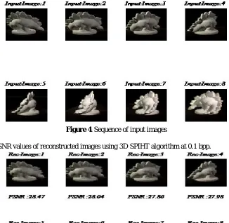
Figure 4. Shows sequence of input images for dataset.

Figure 4. Sequence of input images

Figure 5. Shows PSNR values of reconstructed images using 3D SPIHT algorithm at 0.1 bpp.

(7)

Volume 2, Issue 5, May 2013

Page 390

Figure 6. Shows significant improvement in PSNR values of reconstructed images using 3D SPIHT with PSO

algorithm at 0.1 bpp.

Figure 6 Reconstructed images using 3D SPIHT with PSO algorithm

Figure 7. Shows graph of BPP v/s MSE for 3D SPIHT and 3D SPIHT with PSO algorithm at 0.1 to 0.5 bpp.

Figure 7BPP v/s MSE at 0.1 to 0.5 bpp

Figure 8. Shows graph of BPP v/s PSNR for 3D SPIHT and 3D SPIHT with PSO algorithm at 0.1 to 0.5 bpp.

Figure 8 BPP v/s PSNR at 0.1 to 0.5 bpp

Figure 9. Shows graph of BPP v/s Correlation Coefficient for 3D SPIHT and 3D SPIHT with PSO algorithm at 0.1 to 0.5 bpp.

(8)

Volume 2, Issue 5, May 2013

Page 391

Figure 10. Shows graph of BPP v/s MSSIM for 3D SPIHT and 3D SPIHT with PSO algorithm at 0.1 to 0.5 bpp.

Figure 10 BPP v/s MSSIM at 0.1 to 0.5 bpp

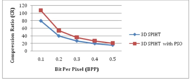
Figure 11. Shows graph of BPP v/s Compression Ratio (CR) for 3D SPIHT and 3D SPIHT with PSO algorithm at 0.1 to 0.5 bpp.

Figure 11 BPP v/s CR at 0.1 to 0.5 bpp

8. C

ONCLUSION

3D SPIHT with PSO algorithm can be used for any image size. When the size of the color image increases, the time required for compression and reconstruction of the image also increases. The algorithm was tested using two color image dataset. The results show that we obtained improvement using 3D SPIHT with PSO algorithm in terms of compression ratio, mean-squared error, and Peak signal to noise ratio, correlation coefficient and multi-scale structural similarity index.

References

[1.]Stephane G. Mallat, “A theory for multi resolution signal decomposition: The wavelet representation” IEEE Trans. Pattern Analysis and Machine Intelligence,vol. 11, no. 7, p. 674–693, Jul.1989.

[2.]A. Said and W. A. Pearlman, "A New fast and efficient image codec based on set partitioning in hierarchical trees", IEEE Transaction On Circuits and Systems for Video Technology, vol. 6, no.3 pp 243-250, Jun. 1996. [3.]F. Khélifi N. Doghmane And T. Bouden, “Compression Of The Color Images By SPIHT Technique”,

[5.]Amar Aggoun, MIEEE, “Compression Of 3D Integral Images Using 3D Wavelet Transform” Journal Of Display Technology, Vol. 7, No. 11, November 2011.

[6.]Hala H. Zayed, Sherin E. Kishk, and Hosam M. Ahmed, “3D Wavelets with SPIHT Coding for Integral Imaging Compression”, IJCSNS International Journal of Computer Science and Network Security, Vol.12 No.1, January 2012.

[7.]Mohammed Hassan, Chakravarthy Bhagvati, “Structural Similarity Measure for ColorImages”, International Journal of Computer Applications (0975 – 8887) Volume 43– No.14, April 2012.

[8.]M.Mohamed Ismail, Dr.K.Baskaran, “Clustering Based Adaptive Image Compression Scheme Using Particle Swarm Optimization Technique”, International Journal of Engineering Science And Technology Vol. 2(10), 2010, 5114-5119.

(9)

Volume 2, Issue 5, May 2013

Page 392

[10.]Michael Clark Weeks, “Architectures For The 3-D Discrete Wavelet Transform”, thesis, spring 1998.

[11.]Tobias Blaser, Stephan Senn, Philipp Stadelmann,“Wavelet-based Compression using the SPIHT Algorithm”,Chip Design Project, 1st April 2006.

[12.]Rafael C. Gonzalez and Richard E Woods, Digital Image Processing, Pearson Education, Inc., 2009.