The Thirty-Third AAAI Conference on Artificial Intelligence (AAAI-19)
Spell Once, Summon Anywhere:
A Two-Level Open-Vocabulary Language Model
Sabrina J. Mielke, Jason Eisner
Department of Computer Science, Johns Hopkins University, Baltimore, MD, USA [email protected], [email protected]
Abstract
We show how the spellings of known words can help us deal with unknown words in open-vocabulary NLP tasks. The method we propose can be used to extend any closed-vocabulary generative model, but in this paper we specifically consider the case of neural language modeling. Our Bayesian generative story combines a standard RNN language model (generating the wordtokensin each sentence) with an RNN-based spelling model (generating the letters in each wordtype). These two RNNs respectively capture sentence structure and word structure, and are kept separate as in linguistics. By in-voking the second RNN to generate spellings for novel words in context, we obtain an open-vocabulary language model. For known words, embeddings are naturally inferred by combining evidence from type spelling and token context. Comparing to baselines (including a novel strong baseline), we beat previous work and establish state-of-the-art results on multiple datasets.
1
Introduction
In this paper, we propose a neural language model that in-corporates a generative model of word spelling. That is, we aim to explain the training corpus as resulting from a pro-cess that first generated a lexicon of word types—the lan-guage’s vocabulary—and then generated the corpus of tokens by “summoning” those types.
Each entry in the lexicon specifies both a syntactic/se-mantic embedding vector and an orthographic spelling. Our model captures the correlation between these, so it can ex-trapolate to predict the spellings ofunknownwords in any syntactic/semantic context. In this sample from our trained English model, the words inthis fontwere unobserved in training data, yet have contextually appropriate spellings:
Following the death of Edward McCartney in1060 , the new definition was transferred to theWDIC ofFullett.
While the fully generative approach is shared by previous Bayesian models of language (e.g., Goldwater, Griffiths, and Johnson (2006)), even those that model characters and words at different levels (Mochihashi, Yamada, and Ueda 2009; Goldwater, Griffiths, and Johnson 2011) have no embeddings and hence no way to relate spelling to usage. They also have
Copyright c2019, Association for the Advancement of Artificial Intelligence (www.aaai.org). All rights reserved.
an impoverished model of sequential structure (essentially,
n-gram models with backoff). We instead employrecurrent neural networksto model both the sequence of words in a sentence and the sequence of characters in a word type, where the latter sequence is conditioned on the word’s embedding. The resulting model achieves state-of-the-art on multiple datasets. It is well-founded in linguistics and Bayesian mod-eling, but we can easily use it in the traditional non-Bayesian language modeling setting by performing MAP estimation.
We begin by concisely stating a first, closed-vocabulary, version of our model in§2, before explaining our motiva-tions from various perspectives in §3. Then §4 motivates and describes a simple way to extend the model to the open-vocabulary setting.§5 contains quantitative and qualitative experiments on multiple language modeling datasets, with implementation details provided in supplementary material. Finally, we clarify the relation of this model to previous work in§6 and summarize our contribution in§7.
2
A joint model of lexicon and text
2.1
Lexemes have embeddings and spellings
We will model text that has already been tokenized, i.e., it is presented as a sequence of word tokensw1,w2, . . ..
We assume that a language’s word types, which we hence-forth calllexemesto avoid confusion, are discrete elements
wof thevocabularyV={1,2, . . .}v . In our model, the observable behavior of the lexemewis determined by two properties: a latent real-valuedembedding e(w)∈Rd, which governs wherewtends to appear, andw’s spellingσ(w)∈Σ∗
(for some alphabet of charactersΣ), which governs how it looks orthographically when it does appear.
We will useeandσto refer to the functions that map each lexemewto its embedding and spelling. Thus the lexicon is specified by(e, σ). Our model1(given fixedvandn) specifies a joint distribution over the lexicon and corpus:
p(θ,e, σ,w1, . . . ,wn) = p(θ)· (1)
∏
w∈Vh
p(e(w))
| {z }
prior on embeddings
·pspell(σ(w)|e(w))
| {z }
spelling model for all types
i
| {z }
lexicon generation
·
n
∏
i=1pLM(wi|~w<i,e)
| {z }
lexeme-level recurrent language model
for all tokens
look up embeddings
look up spellings
N(0,I) e(UNK)
e(1)
e(2)
e(3) RNN cell
RNN cell
RNN cell
t h e
σ(1)
RNN cell
RNN cell
RNN cell
c a t
σ(2)
RNN cell
RNN cell
RNN cell
RNN cell
RNN cell
RNN cell
c h a s e d
σ(3)
~h1
w1 =1 softmax
~h2
RNN
w2 =2 softmax
~h3
RNN
w3
=UNK
softmax
~h4
RNN
w4 =1 softmax
~h5
RNN
... softmax
RNN cell
RNN cell
RNN cell
RNN cell
RNN cell
c a g e d cat
the the ...
σ(w1) σ(w2) s∼pspell(· |~h3) σ(w4)
usage⊥spelling|embedding (conditional independence property) regularize, don’tconstruct
embeddings using spellings
Figure 1: A lexeme’s embedding is optimized to be predictive of the lexeme’s spelling. That spelling is predicted only once (left); every corpus token of that lexeme type (right) simply “summons,” or copies, the type’s spelling. For the novel wordw3
(§4),cagedis preferred over something unpronounceable likexsmfk, but also over the ungrammaticalfurry, because the
hidden state~h3prefers a verb and the spelling model can generalize from the verbchasedending in-edtocaged.
wherepLM(§2.2) andpspell(§2.3) are RNN sequence models
that are parameterized byθ(the dependence is omitted for space reasons), andw1, . . . ,wnis a sequence of word tokens.
Let us unpack this formula. The generative story for the observed training corpus has two steps:
Generate the structure of the language. First draw RNN parametersθ(from a spherical Gaussian). Then draw an embeddinge(w)for each lexemew(from another spherical Gaussian).2Finally, sample a spellingσ(w)for each lexeme
wfrom thepspellmodel, conditioned one(w)(andθ). Generate the corpus. In the final term of (1), generate a
se-quence of lexemesw1, . . . ,wnfrom thepLMmodel (using θ). Applyingσyields the actually observed training corpus
σ(w1), . . . , σ(wn), a sequence of spelled words.
In the present paper we make the common simplifying assumption that the training corpus has no polysemy, so that two word tokens with the same spelling always corre-spond to the same lexeme. We thus assign distinct lexeme numbers1,2, . . . ,v to the different spelling types in the corpus (the specific assignment does not matter). Thus, we have observed the spellingsσ(1), σ(2), . . . , σ(v)of these
vassumed lexemes. We have also observed the actual token sequencew1, . . . ,wnwhere eachwiis a lexeme number.
Given these observations, we trainθandejointly by MAP estimation: in other words, we choose them to (locally) max-imize (1).3 This is straightforward using backpropagation and gradient descent (see Appendix A4on training and Ap-pendix B for implementation and hyperparameter details).
2We will later find the MAP estimates ofθ ande(w), so the
Gaussian priors correspond toL2regularization of these estimates. 3The non-Bayesian view on this is that we maximize the
regu-larized likelihoodof the model given the observations.
4All appendices (supp. material) can be found in the full version
of this paper at https://arxiv.org/abs/1804.08205.
2.2
Modeling word sequences with
p
LMThe final term of (1) is simply a neural language model that uses the embeddingse. It should be stressed thatanysuch neural language model can be used here. We will use the commonly used AWD-LSTM built by Merity, Keskar, and Socher (2017) with their best reported hyperparameters.
2.3
Modeling letter sequences with
p
spellOur model also has to predict the spelling of every lexeme. We modelpspell(σ(w)|e(w))with a vanilla LSTM language
model (Sundermeyer, Schl¨uter, and Ney 2012), this time over characters, using special charactersBOW(beginning of word) andEOW(end of word) to begin and end the sequence.
Our intuition is that in most languages, the spelling of a word tends to weakly reflect categorical properties that are hopefully captured in the embedding. For example, proper names may have a certain form, content words may have to contain at least two syllables (McCarthy and Prince 1999), and past-tense verbs may tend to end with a certain suffix. This is whypspell(σ(w)|e(w))is conditioned on the lexeme’s embedding e(w). We accomplish this by feeding e(w) into LSTMspell as additional input at every step, alongside the
ordinary inputs (the previous hidden stateh~t−1and an
low-dimensional embeddingc~t−1∈Rd 0
of the previous character):
~
ht=LSTMspell h~t−1,[~ct;e(w)]
(2)
As the spelling model tends to overfit to training lexemes (instead of modeling the language’s phonotactics, morphol-ogy, and other conventions), we project the embeddingse(w)
into alower-dimensional spaceto combat this overfitting. We do so by regularizing the four input weight matrices5of LSTMspellwith thenuclear norm(the sum of each matrix’s
5W
singular values; details on it in Appendix C), resulting in a low-rank projection. The nuclear norm (times a positive hy-perparameter) is added to the objective, namely the negative log of Eq. (1), as part of the definition of the−logp(θ)term. This regularizer indeed helps on development data, and it outperformedL2regularization in our pilot experiments.
3
Words, characters, types, and tokens
We now take a step back and discuss our modeling principles. Our model structure above aims to incorporate two perspec-tives that have been neglected in neural language modeling:3.1
A linguistic perspective
Hockett (1960) regardedduality of patterning as a funda-mental property of human language: the formof a word is logically separate from its usage. For example, while
childrenmay be an unusual spelling for a plural noun in
English, it is listed as one in the lexicon, and that grants it all the same privileges as any other plural noun. The syntactic and semantic processes that combine words are blind to its un-usual spelling. In our two-level architecture, this “separation of concerns” holds betweenpspell, which governs wordform,
andpLM, which governs wordusage. A word’s distribution of
contexts is conditionally independent of its spelling, given its embedding, becausepLMdoes not consult spellings but only
embeddings. Prior work doesnotdo this—character-based language models blur the two levels into one.
Half a century earlier, Saussure (1916) discussed the ar-bitrariness of the sign. In our model, pspellhas support on
all ofΣ∗, so any embedding can in principle be paired in the lexicon with any spelling—even if some pairings may be more likelya priorithan others, perhaps because they are more pronounceable or the result of a morphological transfor-mation. In contrast with most prior work that compositionally derives a word’s embedding from its spelling, our model only
prefersa word’s embedding to correlate with its spelling, in order to raise the factorpspell(σ(w)|e(w)). This preference is
merely a regularizing effect that may be overcome by the need to keep thepLMfactors large, particularly for a frequent
word that appears in manypLMfactors and is thus allowed
its own idiosyncratic embedding.
In short, our spelling model isnotsupposed to be able to perfectly predict the spelling. However, it can statistically capture phonotactics, regular and semi-regular inflection, etc.
3.2
A modeling perspective
The distinction between word types (i.e., entries in a vocabu-lary) and tokens (i.e., individual occurrences of these word types in text) is also motivated by a generative (e.g., Bayesian) treatment of language: a lexeme’s spelling isreusedover all its tokens, not generated from scratch for each token.
This means that the term pspell(σ(w)|e(w))appears only
once in (1) for each word typew. Thus, the training of the spelling model is not overlyinfluenced by frequent (and atypical) words liketheanda,6but just as much as by rare
words like deforestation. As a result, pspell learns
6The striking difference between types and tokens is perhaps
most visible withth. It is the most common character bigram in
how typical word types—not typical tokens—are spelled. This is useful in predicting howother typeswill be spelled, which helps us regularize the embeddings of rare word types and predict the spellings of novel word types (§4 below).7
4
Open vocabulary by “spelling”
UNKOur spelling model not only helps us regularize the embed-dings of rare words, but also allows us to handleunknown words, a long-standing concern in NLP tasks.8How?
As a language usually has a fixed known alphabet (so the held-out data will at least not contain unknown characters), a common approach is to model character sequences instead of word sequences to begin with (Sutskever, Martens, and Hinton 2011). However, such a model does not explicitly represent word units, does not respect duality of patterning (§3.1), and thus may have a harder time learning syntactic and semantic patterns at the sentence level. For this reason, several recent approaches have tried to combine character-level modeling with word-character-level modeling (see§6).
Our approach differs from this previous work because we have an explicit spelling model to use. Just as pspellhas an
opinion about how to spell rare words, it also has an opinion about how to spell novel words. This allows the following trick. We introduce a special lexemeUNK, so that the vocab-ulary is nowV={UNK,1,2, . . . ,}v with finite sizev+1. We refine our story of how the corpus is generated. First, the model again predicts a complete sequence of lexemes
w1, . . . ,wn. In most cases,wiis spelled out deterministically asσ(wi). However, ifwi=UNK, then we spell it out by sam-pling frompspell(· |~ei), where~eiis an appropriate embedding, explained below. The downside of this approach is that each
UNKtoken samples a fresh spelling, so multiple tokens of an out-of-vocabulary word type are treated as if they were separate lexemes.
Recall that the spelling model generates a spellinggiven an embedding. So what embedding~eishould we use to gen-erate this unknown word? Imagine the word had been in the vocabulary. Then, if the model had wanted to predict that word,~eiwould have had to have a high dot product with the hidden state of the lexeme-level RNN at this time step,~h. So, clearly, the embedding that maximizes the dot product with the hidden state is just the hidden state itself.9It follows that we should sample the generated spellings∼p(· |~h), using
words of the Penn Treebank as preprocessed by Mikolov et al. (2010) when counting wordtokens, but only appears in 156thplace when counting wordtypes. Looking at trigrams (with spaces) produces an even starker picture: th,the,he are respectively the 1st, 2nd, and 3rdmost common trigrams when looking at tokens, but only the 292nd, 550th, and 812th(out of 5261) when considering types.
7Baayen and Sproat (1996) argue for using only thehapax
legom-ena(words that only appear once) to predict the behavior of rare and unknown words. The Bayesian approach (MacKay and Peto 1995; Teh 2006) is a compromise: frequent word types are also used, but they have no more influence than infrequent ones.
8Often 5–10% of held-out word tokens in language modeling
datasets were never seen in training data. Rates of 20–30% or more can be encountered if the model was trained on out-of-domain data.
9At least, this is the best~e
the current hidden state of the lexeme-level RNN.10 Continuing the generative story, the lexeme-level RNN moves on, but to simplify the inference we feede(UNK)into the lexeme-level RNN to generate the next hidden state, rather than feeding in~h(our guess ofe(σ−1(s))).11
Now we can expand the model described in§2 to deal with sequences containing unknown words. Our building blocks are two old factors from Eq. (1) and a new one:
the lexicon generation ∏w∈V
h
p(e(w))·pspell(σ(w)|e(w))
i
predicts the spellings of in-vocabulary lexemes from their embeddings
the lexeme-level RNN ∏ni=1pLM(wi|~w<i,e)
predicts lexemewifrom the history~w<isummarized as~hi
the spelling of anUNK (new!) pspell(s|~h0)
predicts the spellingsfor anUNKlexeme that appears in a context that led the lexeme-level RNN to hidden state~h0
Using these we can again find the MAP estimate of our parameters, i.e., the (regularized) maximum likelihood (ML) solution, using the posterior that is proportional to the new joint (with the change from Eq. (1) in black):
p(θ,e, σ,s1· · ·sn) = p(θ)· (3)
∏
w∈Vh
p(e(w))·pspell(σ(w)|e(w))
i
·
n
∏
i=1pLM(wi|~w<i,e)·
∏
i:wi=UNKpspell(si|~hi)
wheres1, . . . ,snare the observed spellings that make up the corpus andwi=σ−1(si)if defined, i.e., if there is aw∈ V withσ(w) =si, andwi=UNKotherwise.
The entire model is depicted in Fig. 1. We train it using SGD, computing the different factors of Eq. (3) in an efficient order (implementation details are presented in Appendix A).
5
Experiments
We will now describe the experiments we perform to show that our approach works well in practice.12A detailed discus-sion of all hyperparameters can be found in Appendix B.
5.1
Datasets
We evaluate on two open-vocabulary datasets,WikiText-2
(Merity et al. 2017) and theMultilingual Wikipedia Corpus
(Kawakami, Dyer, and Blunsom 2017).13For each corpus, we
follow Kawakami, Dyer, and Blunsom and replace characters that appear fewer than 25 times by a special symbol3.14
10Note that an in-vocabulary token can now be generated in two
ways, as the spelling of a known lexeme or ofUNK. Appendix D discusses this (largely inconsequential) issue.
11This makes the implementation simpler and faster. One could
also imagine feeding back, e.g., the final hidden state of the speller. 12Code at github.com/sjmielke/spell-once.
13Unlike much previous LM work, we do not evaluate on the Penn
Treebank (PTB) dataset as preprocessed by Mikolov et al. (2010) as its removal of out-of-vocabulary words makes it fundamentally unfit for open-vocabulary language model evaluation.
14This affects fewer than 0.03% of character tokens of WikiText-2
and thus does not affect results in any meaningful way.
WikiText-2 The WikiText-2 dataset (Merity et al. 2017) contains more than 2 million tokens from the English Wikipedia. We specifically use the “raw” version, which is tokenized but has no UNK symbols (since we need the spellings ofallwords).
The results for WikiText-2 are shown in Table 1 in the form of bits per character (bpc). Our full model is denotedFULL. The other rows report on baselines (§5.2) and ablations (§5.3), which are explained below.
Multilingual Wikipedia Corpus The Multilingual Wikipedia Corpus (Kawakami, Dyer, and Blunsom 2017) contains 360 Wikipedia articles in English, French, Spanish, German, Russian, Czech, and Finnish. However, we re-tokenize the dataset, not only splitting on spaces (as Kawakami, Dyer, and Blunsom do) but also by splitting off each punctuation symbol as its own token. This allows us to use the same embedding for a word regardless of whether it has adjacent punctuation. For fairness in comparison, we ensure that our tokenizer preserves all information from the original character sequence (i.e., it is reversible). The exact procedure—which is simple and language-agnostic—is described in Appendix E, with accompanying code.
The results for the MWC are shown in Table 2 in the form of bits per character (bpc).
5.2
Comparison to baseline models
The first baseline model is a purely character-level RNN lan-guage model (PURE-CHAR). It is naturally open-vocabulary (with respect to words; like all models we evaluate, it does as-sume a closed character set). This baseline reaches by far the worst bpc rate on the held-out sets, perhaps because it works at too short a time scale to capture long-range dependencies. A much stronger baseline—as it turns out—is a subword-level RNN language model (PURE-BPE). It models a se-quence ofsubword units, where each token in the corpus is split into one or more subword units byByte Pair Encoding
(BPE), an old compression technique first used for neural machine translation by Sennrich, Haddow, and Birch (2016). This gives a kind of interpolation between a word-level model and a character-level model. The set of subword units is finite and determined from training data, but includes all characters inΣ, making it posssible to explain any novel word in held-out data. The size of this set can be tuned by specifiying the number of BPE “merges.”15To our surprise, it is the strongest competitor to our proposed model, even outperforming it on the MWC. One has to wonder why BPE has not (to our knowl-edge) been tried previously as an open-vocabulary language model, given its ease of use and general applicability.
Notice, however, that even whenPURE-BPEperforms well as a language model, it does not provideword embeddings
to use in other tasks like machine translation, parsing, or en-tailment. We cannot extract the usual static type embeddings
15A segmented example sentence from WikiText-2 is “The
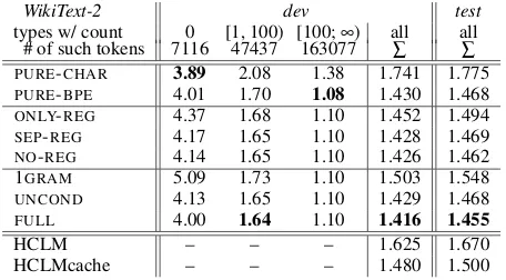
WikiText-2 dev test types w/ count 0 [1, 100) [100;∞) all all # of such tokens 7116 47437 163077 ∑ ∑
PURE-CHAR 3.89 2.08 1.38 1.741 1.775 PURE-BPE 4.01 1.70 1.08 1.430 1.468 ONLY-REG 4.37 1.68 1.10 1.452 1.494 SEP-REG 4.17 1.65 1.10 1.428 1.469 NO-REG 4.14 1.65 1.10 1.426 1.462 1GRAM 5.09 1.73 1.10 1.503 1.548 UNCOND 4.13 1.65 1.10 1.429 1.468
FULL 4.00 1.64 1.10 1.416 1.455
HCLM – – – 1.625 1.670 HCLMcache – – – 1.480 1.500
Table 1: Bits per character (lower is better) on the dev and test set ofWikiText-2for our model and baselines, where
FULLrefers to our main proposed model and HCLM and HCLMcache refer to Kawakami, Dyer, and Blunsom (2017)’s proposed models. All our hybrid models use a vocabulary size of 50000, PURE-BPEuses 40000 merges (both tuned from Fig. 2). All pairwise differences except for those be-tweenPURE-BPE,UNCOND, andSEP-REGare statistically significant (paired permutation test over all 64 articles in the corpus,p<0.011).
from it, nor is it obvious how to create dynamic per-token embeddings like thecontextualized embeddingsof Peters et al. (2018). Our model allows for both, namelye(w)and~hi.
Finally, we also compare against the character-aware model of Kawakami, Dyer, and Blunsom (2017), both with-out (HCLM) and with their additional cache (HCLMcache). To our knowledge, that model has the best previously known performance on theraw (i.e., open-vocab) version of the WikiText-2 dataset, but we see in both Table 1 and Table 2 that our model and thePURE-BPEbaseline beat it.
5.3
Analysis of our model on WikiText-2
Ablating the training objective How important are the various influences onpspell? Recall thatpspellis used to relate
embeddings of in-vocabulary types to their spellings at train-ing time. We can omit thisregularizationof in-vocabulary embeddings by dropping the second factor of the training objective, Eq. (3), which gives theNO-REGablation.pspellis
also trained explicitly to spell outUNKtokens, which is how it will be used at test time. Omitting this part of the training by dropping the fourth factor gives theONLY-REGablation. We can see in Table 1 that neitherNO-REGnorONLY-REG
performs too well (no matter the vocabulary size, as we will see in Figure 2). That is, the spelling model benefits from being trained on both in-vocabulary types andUNKtokens.
To tease apart the effect of the two terms, we evaluate what happens if we use two separate spelling models for the second and fourth factors of Eq. (3), giving us theSEP-REG
ablation. Now the in-vocabulary words are spelled from a different model and do not influence the spelling ofUNK.16
16Though this prevents sharing statistical strength, it might
actu-ally be a wise design ifUNKs are in fact spelled differently (e.g., they tend to be long, morphologically complex, or borrowed).
Interestingly,SEP-REGdoes not perform better thanNO
-REG(in Fig. 2 we see no big difference), suggesting that it is not the “smoothing” of embeddings using a speller model that is responsible for the improvement ofFULLoverNO-REG, but the benefit of training the speller on more data.17
Speller architecture power We also compare our full model (FULL) against two ablated versions that simplify the
spelling model:1GRAM, wherep(σ(w))∝ ∏|iσ=(1w)|q(σ(w)i)(a learned unigram distributionqover characters instead of an RNN) and UNCOND, where p(σ(w))∝pspell(σ(w)|~0), (the
RNN character language model, but without conditioning on a word embedding).
In Table 1, we clearly see that as we go from 1GRAMtoUN
-CONDtoFULL, the speller’s added expressiveness improves the model.
Rare versus frequent words It is interesting to look at bpc broken down by word frequency,18,19shown in Table 1. The first bin contains (held-out tokens of) words that were never seen during training, the second contains words that were only rarely seen (about half of them inV), and the third contains frequent words. Unsurprisingly, rarer words generally incur the highest loss in bpc, although of course their lower frequency does limit the effect on the overall bpc. On the frequent words, there is hardly any difference among the several models—they can all memorize frequent words—except that thePURE-CHARbaseline performs par-ticularly badly. Recall thatPURE-CHARhas to re-predict the spelling of these often irregular types each time they occur. Fixing this was the original motivation for our model.
On the infrequent words,PURE-CHAR continues to per-form the worst. Some differences now emerge among the other models, with ourFULLmodel winning. Even the ab-lated versions of FULL do well, with 5 out of our 6 beat-ing both baselines. The advantage of our systems is that they create lexical entries that memorize the spellings of all in-vocabulary training words, even infrequent ones that are rather neglected by the baselines.
On the novel words, our 6 systems have the same relative ordering as they do on the infrequent words. The surprise in this bin is that the baseline systems do extremely well, with
PURE-BPEnearly matchingFULLandPURE-CHARbeating it, even though we had expected the baseline models to be too biased toward predicting the spelling of frequent words. Note, however, that pspelluses a weaker LSTM thanpLM(fewer
nodes and different regularization), which may explain the difference.
17All this, of course, is only evaluated with the hyperparameters
chosen forFULL. Retuning hyperparameters for every condition might change these results, but is infeasible.
18We obtain the number for each frequency bin by summing the
contextual log-probabilities of the tokens whose types belong in that bin, and dividing by the number of characters of all these tokens. (For thePURE-CHARandPURE-BPEmodels, the log-probability of a token is a sum over its characters or subword units.)
19Low bpc means that the model can predict the tokens in this bin
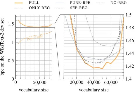
0 50,000 0
0.5 1 1.5
pLM(·)only
vocabulary size
bpc
on
the
W
ikiT
ext-2
de
v
set
20,000 40,000 60,000 1.4 1.42 1.44 1.46 1.48 1.5
vocabulary size FULL PURE-BPE NO-REG ONLY-REG SEP-REG
Figure 2: Bits-per-character (lower is better) on WikiText-2 dev data as a function of vocabulary size. Left: The total cross-entropy is dominated by the third factor of Eq. (3),pLM,
the rest being its fourth factor. Right (zoomed in): baselines.
Vocabulary size as a hyperparameter In Fig. 2 we see that the size of the vocabulary—a hyperparameter of both thePURE-BPEmodel (indirectly by the number of merges used) and ourFULLmodel and its ablations—does influence results noticeably. There seems to be a fairly safe plateau when selecting the 50000 most frequent words (from the raw WikiText-2 vocabulary of about 76000 unique types), which is what we did for Table 1. Note that atanyvocabulary size, both models perform far better thanPURE-CHAR, whose bpc of 1.775 is far above the top of the graph.
Figure 2 also shows that as expected, the loss of theFULL
model (reported as bpc on the entire dev set) is made up mostly of the cross-entropy ofpLM. This is especially so for
larger vocabularies, where very fewUNKs occur that would have to be spelled out usingpspell.
5.4
Results on the multilingual corpus
We evaluated on each MWC language using the system and hyperparameters that we had tuned on WikiText-2 develop-ment data. Even the vocabulary size stayed fixed at 60000.20
Frustratingly, lacking tuning to MWC, we do not outper-form our own (novel) BPE baseline on MWC. We peroutper-form at most equally well, even when leveling the playing field through proper tokenization (§5.1). Nevertheless we outper-form the best model of Kawakami, Dyer, and Blunsom (2017) on most datasets, even when using the space-split version of the data (which, as explained in§5.1, hurts our models).
Interestingly, the datasets on which we lose toPURE-BPE
are Czech, Finnish, and Russian—languages known for their morphological complexity. Note thatPURE-BPEgreatly ben-efits from the fact that these languages have a
concatena-20Bigger vocabularies require smaller batches to fit our GPUs,
so changing the vocabulary size would have complicated fair com-parisons across methods and languages, as the batch size has a large influence on results. However, the optimal vocabulary size is presumably language- and dataset-dependent.
tive morphological system unlike Hebrew or Arabic. Ex-plicitly incorporating morpheme-level information into our
FULLmodel might be useful (cf. Matthews, Neubig, and Dyer (2018)). Our present model or its current hyperparame-ter settings (especially the vocabulary size) might not be as language-agnostic as we would like.
5.5
What does the speller learn?
Finally, Table 3 presents non-cherry-picked samples from
pspell, after training ourFULLmodel on WikiText-2. pspell
seems to know how to generate appropriate random forms that appear to have the correct part-of-speech, inflectional ending, capitalization, and even length.
We can also see how the speller chooses to create formsin context, when trying to spell outUNKgiven the hidden state of the lexeme-level RNN. The model knowswhenandhow
to generate sensible years, abbreviations, and proper names, as seen in the example in the introduction (§1).21 Longer,
non-cherry-picked samples for several of our models can be found in Appendix F.
6
Related work
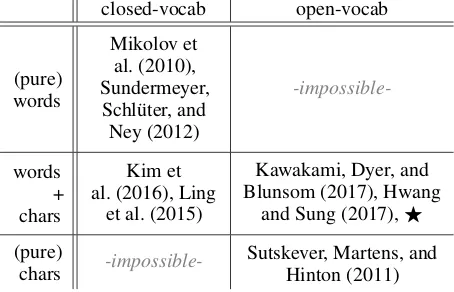
Unlike most previous work, we try tocombineinformation about words and characters to achieve open-vocabulary mod-eling. The extent to which previous work achieves this is as shown in Table 4 and explained in this section.
Mikolov et al. (2010) first introduced a purely word-level (closed-vocab) RNN language model (later adapted to LSTMs by Sundermeyer, Schl¨uter, and Ney (2012)). Sutskever, Martens, and Hinton (2011) use an RNN to generate pure character-level sequences, yielding an open-vocabulary language model, but one that does not make use of the existing word structure.
Kim et al. (2016) and Ling et al. (2015) first combined the two layers by deterministically constructing word embed-dings from characters (training the embedding function on tokens, not types, to “get frequent words right”—ignoring the issues discussed in§3). Both only perform language modeling with a closed vocabulary and thus use the subword informa-tion only to improve the estimainforma-tion of the word embeddings (as has been done before by dos Santos and Zadrozny (2014)).
Another line of work instead augments a character-level RNN with word-level “impulses.” Especially noteworthy is the work of Hwang and Sung (2017), who describe an archi-tecture in which character-level and word-level models run in parallel from left to right and send vector-valued messages to each other. The word model sends its hidden state to the char-acter model, which generates the next word, one charchar-acter at a time, and then sends its hidden state back to update the state of the word model. However, as this is another example ofconstructingword embeddings from characters, it again overemphasizes learning frequent spellings (§3.2).
Finally, the most relevant previous work is the (indepen-dently developed) model of Kawakami, Dyer, and Blun-som (2017), where each word has to be “spelled out” using a character-level RNN if it cannot be directly copied from the
21Generated at temperatureT=0.75 from a
MWC en fr de es cs fi ru
dev test dev test dev test dev test dev test dev test dev test
space-split
#types→merges/
vocab 195k→60k 166k→60k 242k→60k 162k→60k 174k→60k 191k→60k 244k→60k
PURE-BPE 1.50 1.439 1.40 1.365 1.49 1.455 1.46 1.403 1.92 1.897 1.73 1.685 1.68 1.643 FULL 1.57 1.506 1.48 1.434 1.66 1.618 1.53 1.469 2.27 2.240 1.93 1.896 2.00 1.969 HCLM 1.68 1.622 1.55 1.508 1.66 1.641 1.61 1.555 2.07 2.035 1.83 1.796 1.83 1.810 HCLMcache 1.59 1.538 1.49 1.467 1.60 1.588 1.54 1.498 2.01 1.984 1.75 1.711 1.77 1.761
tok
enize
#types→merges/
vocab 94k→60k 88k→60k 157k→60k 93k→60k 126k→60k 147k→60k 166k→60k
PURE-BPE 1.45 1.386 1.36 1.317 1.45 1.414 1.42 1.362 1.88 1.856 1.70 1.652 1.63 1.598 FULL 1.45 1.387 1.36 1.319 1.51 1.465 1.42 1.363 1.95 1.928 1.79 1.751 1.74 1.709
Table 2: Bits per character (lower is better) on the dev and test sets of theMWCfor our model (FULL) and Kawakami, Dyer, and Blunsom (2017)’s HCLM and HCLMcache, both on the space-split version used by Kawakami, Dyer, and Blunsom (2017) and the more sensibly tokenized version. Values across all rows are comparable, since the tokenization is reversible and bpc is still calculated w.r.t. the number of characters in the original version. All our models did not tune the vocabulary size, but use 60000.
σ(w) s∼pspell(· |e(w))
grounded stipped
differ coronate
Clive Dickey
Southport Strigger
Carl Wuly
Chants Tranquels
valuables migrations
Table 3: Take an in-vocabulary wordw(non-cherry-picked), and compareσ(w)to a random spellings∼pspell(· |e(w)).
closed-vocab open-vocab
(pure) words
Mikolov et al. (2010), Sundermeyer, Schl¨uter, and
Ney (2012)
-impossible-words + chars
Kim et al. (2016), Ling
et al. (2015)
Kawakami, Dyer, and Blunsom (2017), Hwang
and Sung (2017),F
(pure)
chars
-impossible-Sutskever, Martens, and Hinton (2011)
Table 4: Contextualizing this work (F) on two axes
recent past. As in Hwang and Sung (2017), there is no fixed vocabulary, so words that have fallen out of the cache have to be re-spelled. Our hierarchical generative story—specifically, the process that generates the lexicon—handles the re-use of words more gracefully. Our speller can then focus on rep-resentative phonotactics and morphology of the language instead of generating frequent function words liketheover and over again. Note that the use case that Kawakami et al. originally intended for their cache, the copying of highly infrequent words likeNoriegathat repeat on a very local scale (Church 2000), is not addressed in our model, so adding their cache module to our model might still be beneficial.
Less directly related to our approach of improving lan-guage models is the work of Bhatia, Guthrie, and Eisen-stein (2016), who similarly realize that placing priors on word embeddings is better than compositional construction, and Pinter, Guthrie, and Eisenstein (2017), who prove that the spelling of a word shares information with its embedding. Finally, in the highly related field of machine transla-tion, Luong and Manning (2016) before the re-discovery of BPE proposed an open-vocabulary neural machine trans-lation model in which the prediction of anUNKtriggers a character-level model as a kind of “backoff.” We provide a proper Bayesian explanation for this trick and carefully ab-late it (calling itNO-REG), finding that it is insufficient, and that training on types (as suggested by far older research) is more effective for the task of language modeling.
7
Conclusion
We have presented a generative two-level open-vocabulary language model that can memorize spellings and embeddings of common words, but can also generate new word types in context, following the spelling style of in- and out-of-vocabulary words. This architecture is motivated by linguists’ “duality of patterning.” It resembles prior Bayesian treatments
of type reuse, but with richer (LSTM) sequence models. We introduced a novel, surprisingly strong baseline, beat it by tuning our model, and carefully analyzed the performance of our model, baselines, and a variety of ablations on multi-ple datasets. The conclusion is simmulti-ple: pure character-level modeling is not appropriate for language, nor required for an open vocabulary. Our ablations show that the generative story our model is based on is superior to distorted or simplified models resembling previous ad-hoc approaches.
Acknowledgments
This material is based upon work supported by the Na-tional Science Foundation under Grant No. 1718846. Part of the research made use of computational resources at the Maryland Advanced Research Computing Center (MARCC). The authors would like to thank Benjamin Van Durme and Yonatan Belinkov for helpful suggestions on experiments, and Annabelle Carrell as well as the anonymous reviewers for their suggestions on improving the exposition.
References
Baayen, H., and Sproat, R. 1996. Estimating lexical priors for low-frequency syncretic forms. Computational Linguistics 22(2):155–166.
Bhatia, P.; Guthrie, R.; and Eisenstein, J. 2016. Morphologi-cal priors for probabilistic neural word embeddings. In Proceed-ings of the 2016 Conference on Empirical Methods in Natural Language Processing, 490–500. Austin, Texas: Association for Computational Linguistics.
Church, K. W. 2000. Empirical estimates of adaptation: The chance of two Noriegas is closer top/2 thanp2. InProceedings of the 18th Conference on Computational Linguistics - Volume 1, 180–186. Association for Computational Linguistics.
dos Santos, C., and Zadrozny, B. 2014. Learning character-level representations for part-of-speech tagging. InProceedings of the 31st International Conference on Machine Learning (ICML-14), 1818–1826.
Goldwater, S.; Griffiths, T. L.; and Johnson, M. 2006. Contextual dependencies in unsupervised word segmentation. InProc. of COLING-ACL.
Goldwater, S.; Griffiths, T. L.; and Johnson, M. 2011. Producing power-law distributions and damping word frequencies with two-stage language models. Journal of Machine Learning Research 12(Jul):2335–2382.
Hockett, C. F. 1960. The origin of speech. Scientific American 203(3):88–97.
Hwang, K., and Sung, W. 2017. Character-level language mod-eling with hierarchical recurrent neural networks. InAcoustics, Speech and Signal Processing (ICASSP), 2017 IEEE Interna-tional Conference on, 5720–5724. IEEE.
Kawakami, K.; Dyer, C.; and Blunsom, P. 2017. Learning to create and reuse words in open-vocabulary neural language mod-eling. InProceedings of the 55th Annual Meeting of the ACL (Volume 1: Long Papers), 1492–1502. Vancouver, Canada: Asso-ciation for Computational Linguistics.
Kim, Y.; Jernite, Y.; Sontag, D.; and Rush, A. M. 2016. Character-aware neural language models. InAAAI, 2741–2749.
Kudo, T. 2018. Subword regularization: Improving neural net-work translation models with multiple subword candidates. In Proceedings of the 56th Annual Meeting of the Association for Computational Linguistics (Volume 1: Long Papers), 66–75. Mel-bourne, Australia: Association for Computational Linguistics. Ling, W.; Dyer, C.; Black, A. W.; Trancoso, I.; Fermandez, R.; Amir, S.; Marujo, L.; and Luis, T. 2015. Finding function in form: Compositional character models for open vocabulary word repre-sentation. InProceedings of the 2015 Conference on Empirical Methods in Natural Language Processing, 1520–1530. Lisbon, Portugal: Association for Computational Linguistics.
Luong, M.-T., and Manning, C. D. 2016. Achieving open vo-cabulary neural machine translation with hybrid word-character
models. InProceedings of the 54th Annual Meeting of the ACL (Volume 1: Long Papers), 1054–1063. Berlin, Germany: Associ-ation for ComputAssoci-ational Linguistics.
MacKay, D. J. C., and Peto, L. C. B. 1995. A hierarchical Dirich-let language model. Journal of Natural Language Engineering 1(3):289–308.
Matthews, A.; Neubig, G.; and Dyer, C. 2018. Using morpholog-ical knowledge in open-vocabulary neural language models. In HLT-NAACL.
McCarthy, J., and Prince, A. 1999. Faithfulness and identity in prosodic morphology. In Kager, R.; van der Hulst, H.; and Zonn-eveld, W., eds.,The Prosodic Morphology Interface. Cambridge University Press. 269–309.
Merity, S.; Xiong, C.; Bradbury, J.; and Socher, R. 2017. Pointer sentinel mixture models. InProc. International Conference on Learning Representations.
Merity, S.; Keskar, N. S.; and Socher, R. 2017. Regulariz-ing and optimizRegulariz-ing LSTM language models. arXiv preprints abs/1708.02182.
Mikolov, T.; Karafi´at, M.; Burget, L.; ˇCernock`y, J.; and Khudan-pur, S. 2010. Recurrent neural network based language model. InEleventh Annual Conference of the International Speech Com-munication Association.
Mochihashi, D.; Yamada, T.; and Ueda, N. 2009. Bayesian un-supervised word segmentation with nested pitman-yor language modeling. InProceedings of the Joint Conference of the 47th Annual Meeting of the ACL and the 4th International Joint Con-ference on Natural Language Processing of the AFNLP, 100–108. Suntec, Singapore: Association for Computational Linguistics. Peters, M. E.; Neumann, M.; Iyyer, M.; Gardner, M.; Clark, C.; Lee, K.; and Zettlemoyer, L. 2018. Deep contextualized word representations.Proc. International Conference on Learning Rep-resentations.
Pinter, Y.; Guthrie, R.; and Eisenstein, J. 2017. Mimicking word embeddings using subword rnns. InProceedings of the 2017 Con-ference on Empirical Methods in Natural Language Processing, 102–112. Copenhagen, Denmark: Association for Computational Linguistics.
Saussure, F. d. 1916. Course in General Linguistics. Columbia University Press. English edition of June 2011, based on the 1959 translation by Wade Baskin.
Sennrich, R.; Haddow, B.; and Birch, A. 2016. Neural machine translation of rare words with subword units. InProceedings of the 54th Annual Meeting of the ACL (Volume 1: Long Papers), 1715–1725. Berlin, Germany: Association for Computational Linguistics.
Sundermeyer, M.; Schl¨uter, R.; and Ney, H. 2012. LSTM neural networks for language modeling. InThirteenth Annual Confer-ence of the International Speech Communication Association. Sutskever, I.; Martens, J.; and Hinton, G. 2011. Generating text with recurrent neural networks. In Getoor, L., and Scheffer, T., eds., Proceedings of the 28th International Conference on Ma-chine Learning (ICML-11), ICML ’11, 1017–1024. New York, NY, USA: ACM.