The Thirty-Third AAAI Conference on Artificial Intelligence (AAAI-19)
Inter-Class Angular Loss for Convolutional Neural Networks
Le Hui,
†Xiang Li,
†Chen Gong,
†Meng Fang,
‡Joey Tianyi Zhou,
§Jian Yang
†∗†PCA Lab, Key Lab of Intelligent Perception and Systems for High-Dimensional Information of Ministry of Education
†Jiangsu Key Lab of Image and Video Understanding for Social Security
†School of Computer Science and Engineering, Nanjing University of Science and Technology, Nanjing, China
‡Tencent AI Lab, Shenzhen, China §Institute of High Performance Computing , Singapore
{le.hui, xiang.li.implus, chen.gong, csjyang}@njust.edu.cn, [email protected], [email protected]
Abstract
Convolutional Neural Networks (CNNs) have shown great power in various classification tasks and have achieved re-markable results in practical applications. However, the dis-tinct learning difficulties in discriminating different pairs of classes are largely ignored by the existing networks. For instance, in CIFAR-10 dataset, distinguishing cats from dogs is usually harder than distinguishing horses from ships. By carefully studying the behavior of CNN models in the training process, we observe that the confusion level of two classes is strongly correlated with their angular separability in the feature space. That is, the larger the inter-class angle is, the lower the confusion will be. Based on this observation, we propose a novel loss function dubbed “Inter-Class Angular Loss” (ICAL), which explicitly models the class correlation and can be directly applied to many existing deep networks. By minimizing the proposed ICAL, the networks can effec-tively discriminate the examples in similar classes by en-larging the angle between their corresponding class vectors. Thorough experimental results on a series of vision and non-vision datasets confirm that ICAL critically improves the discriminative ability of various representative deep neural networks and generates superior performance to the original networks with conventional softmax loss.
Introduction
Over the past few years, Convolutional Neural Networks (CNNs) have been successfully applied to various image analysis tasks and gradually become one of the most pow-erful machine learning approaches nowadays. In particular, CNNs have achieved state-of-the-art results for a wide range of challenging tasks such as object recognition (Krizhevsky, Sutskever, and Hinton 2012; Li et al. 2016), hand-written digit recognition (LeCun et al. 1989), image classification (Deng et al. 2009; Gong et al. 2016; 2017), natural language processing (Kim 2014; Lai et al. 2015; Liu, Qiu, and Huang 2016; Wang et al. 2017), etc.
Generally, the key components of a CNN for visual classi-fication tasks includes stacked convolutional layers, pooling layers, and a linear matrix with the softmax function. The earliest CNN can be dated back to LeNet5 (LeCun et al. 1998), which has only five layers. Recently, He et al.(He
∗
Corresponding author
Copyright c2019, Association for the Advancement of Artificial Intelligence (www.aaai.org). All rights reserved.
et al. 2016a) introduced the deep residual network with more than 1000 layers, which is a huge breakthrough in training extreme deep neural networks. Other typical CNNs including (Simonyan and Zisserman 2015; Szegedy et al. 2015; Srivastava, Greff, and Schmidhuber 2015; Szegedy et al. 2016; He et al. 2016a; Xie et al. 2017; Huang et al. 2017; Szegedy et al. 2017) have exhibited strong learning ability and obtained superior performance to traditional learning approaches on a variety of tasks. In summary, the classical CNNs’ structure can be viewed as a convolutional feature learning machine supervised by the softmax loss. The convolutional layers extract the discriminative features of an input image, and send the features into the softmax layer for classification.
However, in classical CNNs’ structure, the softmax func-tion ignores the distinct difficulties for discriminating the examples in different categories. In fact, the inter-class similarities between different categories are very different. For instance, in CIFAR-10 (Krizhevsky and Hinton 2009) dataset, distinguishing cats and dogs is usually harder than distinguishing horses and ships for CNNs, as the cats often share many similar local patterns with dogs. Unfortunately, the softmax operation fails to explicitly consider the dif-ferent distinguishability of inter-class pairs, which is an important issue that has been largely neglected.
By a series of exploratory experiments, it is observed that there exists a correlation between the angle of two classes and the difficulty in correctly distinguishing them. As shown in Fig. 1, the smaller the angle of a pair of classes is, the harder will be for a network to distinguish them. From the angular matrix shown in Fig. 1(a), we see that the angle θcat,dogis smaller than angleθdog,plane, which is consistent
with our general understanding that separating cats and dogs is actually more difficult than distinguishing between dogs from planes.
final
0.8
0.6
0.4
0.2
0.0
100°
80°
60°
40°
20°
0°
Con
fu
sion
Ma
tr
ix
An
gu
lar
Ma
tri
x
P1 P2
>100°
(a) (b) (c) (d)
P1
P2
𝑾𝑑𝑜𝑔
𝑾𝑐𝑎𝑡
𝜽 = 72°
𝑾𝑑𝑜𝑔
𝑾𝑐𝑎𝑡
𝜽 = 83°
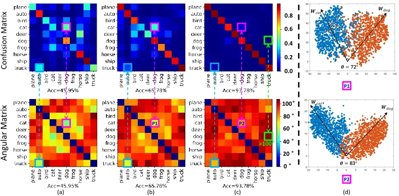
Figure 1: The visualizations of Confusion Matrix and Angular Matrix of ResNet on CIFAR-10 (Krizhevsky and Hinton 2009) dataset. The (a), (b) and (c) denote the different states of the model with the corresponding confusion matrix and angular matrix between pairs of categories, respectively. Additionally, (d) shows the class vectors between the “cat” and “dog” with the corresponding angles. As shown in (a) to (c), when the angle between the category pairs increases, the confusion level between them decreases. In (d), the angle between the class vectors of hard example “cat” and “dog” increases, leading to the improvement of discriminability between them.
between a pair of classes will gradually decrease with the increase ofθ. By applying the angular factor into the loss function ICAL, our method is able to drive the inter-class angle to be as large as possible.
Our numerical experiments are performed by applying the proposed ICAL to several popular deep networks. The re-sults of corresponding networks can be effectively enhanced as revealed by rich experiments on various tasks related to image and text. We visualize the class scores between hard category pairs to demonstrate that the two similar categories are indeed separated by our ICAL. Therefore, our proposed ICAL is critical to boosting the discriminability of various deep networks, leading to the improved final performance for a variety of classification tasks.
Related Works
In the literature of machine learning and mathematical opti-mization, a range of loss functions such as contrastive loss (Hadsell, Chopra, and LeCun 2006), triplet loss (Schroff, Kalenichenko, and Philbin 2015), center loss (Wen et al. 2016) and large-margin loss (Liu et al. 2016) have been proposed. However, these approaches focus more on the intra-class compactness, and partially ignore the distinct difficulties in discriminating different category pairs.
In the triplet loss process, a three tuple containing three examples xa, xp (the same class of xa), and xn (the
different class ofxa) is built, which is to make the distance
between the feature expressions ofxa andxp as small as
possible and the distance between the feature expressions of xa andxnas large as possible. Triplet loss is usually used
at the individual level for fine-grained identification. Slow convergence and overfitting problem exist in its applications,
and the establishment of three tuple is also a heavy cost.
Very recently, the principle of center loss (Wen et al. 2016) is presented based on the softmax loss. By maintain-ing a clustermaintain-ing center in the feature space of each category from the training set, center loss makes the samples in the same class closer to their clustering center during the training, in order to guarantee the intra-class compactness. It only considers intra-class compactness without taking into enough account of distinct confusion levels between different class pairs.
Furthermore, the large-margin softmax (L-Softmax) loss (Liu et al. 2016) is an extension of softmax loss as well. It is done by incorporating a preset constantmmultiplying with the angle θ between the sample’s feature vector and the ground truth class vector, hence making the samples concentrated into their ground truth vectors. The large-margin aims to narrow the angle between a sample and its corresponding class vector. However, this method still has several drawbacks. For one thing, L-Softmax Loss utilizes the binomial approximation to compute the cosine value of inter-class angle, in which only the first two terms are preserved and the remaining high-order terms are directly dropped. Therefore, the finally optimized result is inaccurate and may not be the real optimal solution. For another, the parameter m which explicitly controls the inter-class angle is only allowed to choose from discrete values, so the practical parameter tuning could be difficult and the peak performance might be missed. Furthermore, the optimalm is strongly related to the relative magnitude of class vectors W1andW2. Unfortunately, these class vectors are unknown
Table 1: The top three minimal angles of the angular matrix at four different periods along with the overall performances.Acc is short for Accuracy. As the angle between every category pairs increases, the overall accuracy improves.
Periods Epoch 4 (Acc 72%) Epoch 33 (Acc 85%) Epoch 100 (Acc 90%) Epoch 188 (Acc 95%) Top 3 71◦(dog/cat) 75◦(dog/cat) 76◦(truck/auto) 83◦(truck/auto) minimal 72◦(truck/auto) 75◦(truck/auto) 79◦(dog/cat) 86◦(dog/cat)
angles 80◦(ship/plane) 83◦(ship/plane) 86◦(ship/plane) 88◦(ship/plane)
Figure 2: Classification accuracies (%) of different methods on CIFAR-10 dataset. The horizontal axis represents the tuning parameters for different methods (i.e.the mfor L-Softmax Loss and λ for our ICAL). Note that the value of parameter m is discrete, while our parameter λ is continuous.
any approximate calculations and the parameter governing the inter-class angle is continuous, therefore the output of our method is accurate and the produced inter-class angle can be more easily controlled. An intuitive comparison of the two losses under different values of tuning parameter is presented in Fig. 2. We see that compared to the L-Softmax Loss, the performance of our method is not sensitive to inter-class angular parameter (i.e. λin Eq. (3)). Therefore, the selection of parameter in our method is much easier than L-Softmax Loss. The reason lies in that we have normalized the class vectors in advance. Furthermore, the backpropagation process induced by L-Softmax Loss cannot be directly implemented by the existing neural network toolkit such as Caffe and Tensorflow, as the gradient should be manually calculated. In contrast, our ICAL is quite simple of which the backpropagation process can be automatically implemented without writing any code.
As a result, the ICAL is specifically designed in this paper to enhance the discriminative ability between hard category pairs to improve the classification performance of CNNs. We use the experimental results and the corresponding analysis to show how our Inter-Class Angular Loss works well.
Relationship between Inter-Class Angle and
Learning Difficulty
As illustrated above, the softmax loss does not explicitly discriminate distinct difficulties in inter-classes. In contrast, our proposed ICAL is able to obtain discriminative learning results by enlarging the angle between confusing classes. First, to give a direct motivation, we conduct a series of explorations in this section.
On CIFAR-10 (Krizhevsky and Hinton 2009) dataset,
as shown in Fig. 1, we visualize the confusion matrix and angular matrix on the test set during different training periods. In the confusion matrix, the larger the element is, the more confusion between the corresponding two classes arises. In the angular matrix, the smaller the element is, the similar the two classes are. One can see that every diagonal element of the angular matrix is zero as it represents the self-similarity of a certain class.
In Fig. 1(a), it is very clear that θcat,dog ≤ θdog,plane
and θtruck,auto ≤ θtruck,deer, and the confusion level of
cats and dogs, truck and auto are crucially high from the corresponding confusion matrix. The level of confusion is typically low, when the angle of some class pairs is larger than 100 degrees (e.g. θtruck,dog > 100◦ in Fig. 1(c)).
As shown in Fig. 1(d), we give a visualization of class vectors between “cat” and “dog”, which indicates that with the increase of angles and the accuracies increase. The confusion matrix and angular matrix are almost synchronous in the process of their evolutions from (a) to (c). To further confirm the relationship, we calculate the top three minimal angles with the corresponding category pairs as shown in Tab. 1. It shows that with the improvement of the overall angle of the class pairs, the accuracy between class pairs increases. By combing Tab. 1 with Fig. 1, it is clear that the smaller the angle, the harder it is to distinguish the corresponding classes.
Thus, our work tries to explicitly widen the angle of inter-classes to improve the discriminating ability of hard category pairs, as well as the generalizability of model.
Methodology
Preliminaries
We describe the discriminative difficulty between the two classes to improve the traditional softmax loss via introduc-ing the cosine distance. Given the examplexiwith the label
yi, the original softmax loss can be written as
L= 1
N
XN
i=1Li= 1
N
XN
i=1−log
efyi
PK
j=1efj !
, (1)
wherefjdenotes thej-th element (j= 1,2,· · · , KwithK
being the number of classes) of the class score vectorf, and Nis the number of training samples.fyican also be written
asfyi =W
T
yixiwhereWyiis theyi-th column ofW. Here
W is the weight of the last fully connected layer in CNN. We further expand fyi as fyi = kWyik2kxik2cos (θyi)
whereθyi is the angle between the class vectorWyi and the
examplexi. Therefore, our intuition is that the separability
between the examplexiand the class vectorWyican be
an angular component with cosine similaritycos (θyi).
Sim-ilarly, we may define the similarity between the two classes c0 and c1 as WcT0Wc1 = kWc0k2kWc1k2cos (θc0,c1),
where Wc0 and Wc1 correspond to the class vectors of
class c0 and c1, and θc0,c1 is the angle between the two
class vectorsWc0andWc1. Therefore, in our approach, the
angle between two classesci andcj (ci, cj = 1,2,· · ·, K)
is modeled by θci,cj, which can be computed by θci,cj = arccos(WT
ciWcj/ kWcik2kWcjk2
). HereWci andWcj
represent the class vectors of classciandcj, respectively.
ICAL
According to the above explanation, the angle of the two classes is defined as the angle between their corresponding class vectors. The cosine function is used to measure the angle of class vectors according to its property of mono-tonically decreasing in [0◦,180◦]. The smaller the cosine value is, the larger the inter-class angle will be. To increase the angle between the classes, we minimize the cos (θi,j)
(i, j= 1,2,· · ·, K) for optimization. Therefore, the average sum of cosine similarity (dubbed “AverageSim”) between pairs of classes can be formulated as
AverageSim= 1
K2
XK
i,j=1cos θi,j
. (2)
By combing softmax loss with the defined AverageSim, the preliminary ICAL is
ICAL θi,j
= 1
N
XN
i=1−log
efyi
PK
j=1efj !
+λ 1 K2
XK
i,j=1cos θi,j
, (3)
where λ is the free parameter that needs to be manually adjusted.
Moreover, Eq. (3) can be further simplified by expanding the last term. By usingθi,j to represent the angle between
the class vectorswiandwj(wiandwjare thei-th andj-th
rows ofW), we have
XK
i,j=1cos (θi,j) =
XK
i,j=1w T iwj/
kwik2
wj 2 . (4) Unfortunately, the complexity for computing Eq. (4) is as high asO(K2). With the increase of the number of classes K, the complexity of computing Eq. (4) will grow by square, which affects the effectiveness in the presence of a large amount of categories. By row-normalizingW and denoting vi =wi/kwik2, Eq. (4) is expressed as
XK
i,j=1cos (θi,j) =
XK
i,j=1v T
ivj, (5)
whereviandvj are the normalized class vectors. Note that
wheni=j, the cosine value of corresponding class vectors is always 1. Therefore, we only consider the case ofi6=jin Eq. (5), namely
XK
i,j=1(i6=j)v T ivj=
XK
i=1v T i
XK
j=1vj−
XK
i=1v T ivi,
(6)
whereviTvi= 1. Thus the cosine function is reduced to
XK
i,j=1(i6=j)cos (θi,j) =
XK
i=1v T i
XK
j=1vj−K. (7)
Comparing Eq. (4) and Eq. (7), the complexity for comput-ing cosine function is reduced from O(K2) toO(K). By
putting Eq. (3) and Eq. (7) together and ignoring the constant number, ICAL can be eventually written as
ICAL(θi,j) =L+λ
1
K2
XK
i=1v T i
XK
j=1vj. (8)
Optimization
The forward and backward propagation rule of our ICAL is quite straightforward. Therefore, the conventional stochastic gradient descent can be used for the optimization process.
By comparing ICAL with the original softmax loss, the only difference is that ICAL have an extra cosine loss (i.e. the second term in Eq. (8)), namely
D=λ 1 K2
XK
i=1v T i
XK
i=1vi, vi=wi/kwik2. (9)
As a result, we only need to consider D in deriving the forward and backward propagation rule. For backward prop-agation, we use the chain rules to calculate partial derivatives ofDtovi, which arrives at
∂D ∂vi
=λ 2
K2
XK
i=1vi. (10)
Note that each row of W should be normalized as men-tioned above. To achieve this, in Eq. (9), we rescale the weight matrixW during the feed forward process. Note that such weight normalization is nested in the network, rather than explicitly conducted after each iteration. Additionally, we need to calculate the partial derivative of each element of vitowiin backward propagation, which is very similar to
Eq. (10) and thus is omitted here.
Discussion
The proposed ICAL has several nice properties:
• The ICAL is a general loss function and can be applied to many typical deep neural networks such as data aug-mentation, pooling functions and other modified network architectures.
• The ICAL has a clear geometric explanation, and mini-mizing it helps to reduce the confusion level between dif-ferent classes, by which the distinguishability of network can be substantially enhanced.
• The ICAL has only one parameterλ to tune, making it very convenient for practical use.
Experiments
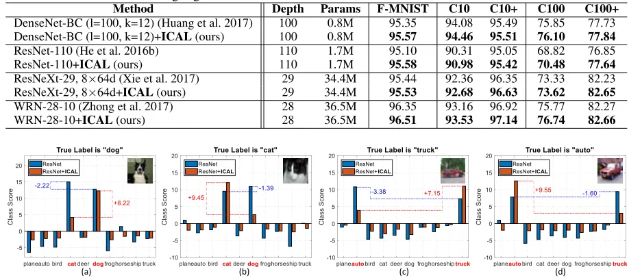
Table 2: Classification accuracies (%) of various methods on Fashion-MNIST, CIFAR-10 and CIFAR-100 datasets (“F-MNIST”, “C10”, “C100” for short, respectively). The mark “+” indicates that the standard data augmentation (crop and/or flip) is used. The better results are highlighted inbold.
Method Depth Params F-MNIST C10 C10+ C100 C100+
DenseNet-BC (l=100, k=12) (Huang et al. 2017) 100 0.8M 95.35 94.08 95.49 75.85 77.73
DenseNet-BC (l=100, k=12)+ICAL(ours) 100 0.8M 95.57 94.46 95.51 76.10 77.84
ResNet-110 (He et al. 2016b) 110 1.7M 95.10 90.31 95.05 68.82 76.85
ResNet-110+ICAL(ours) 110 1.7M 95.58 90.98 95.42 70.48 77.64
ResNeXt-29, 8×64d (Xie et al. 2017) 29 34.4M 95.44 92.36 96.35 73.33 82.23
ResNeXt-29, 8×64d+ICAL(ours) 29 34.4M 95.53 92.68 96.63 73.62 82.65
WRN-28-10 (Zhong et al. 2017) 28 36.5M 96.35 93.16 96.92 75.77 82.27
WRN-28-10+ICAL(ours) 28 36.5M 96.51 93.53 97.14 76.74 82.66
(a) (b) (c) (d)
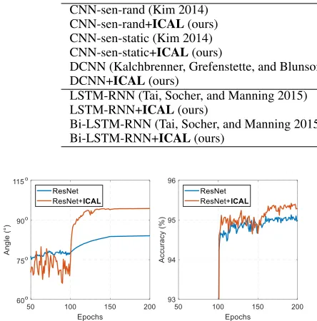
Figure 3: Class scores of confused categories on CIFAR-10 dataset generated by softmax and ICAL.
Experiments on Vision Datasets
Datasets Description Three challenging image classifica-tion datasets are used for the experiments, which include
• Fashion-MNIST (Xiao, Rasul, and Vollgraf 2017) is a dataset of clothes images containing a training set of 60K examples and a test set of 10K examples. Each example is a 28×28 grayscale image, associated with a label from 10 categories. It is intended to replace the original MNIST (LeCun et al. 1998) dataset with Fashion-MNIST for machine learning algorithms. Fashion-MNIST includes many similar categories of clothes like “Shirt” and “T-Shirt/Top”, which are very difficult to discriminate.
• CIFAR(Krizhevsky and Hinton 2009) dataset consists of totally 60K colored natural scene images with the resolu-tion of 32×32. The training set and test set contain 50K images and 10K images, respectively. CIFAR contains two versions, namely CIFAR-10 including 10 classes and CIFAR-100 including 100 classes. Following (Huang et al. 2017), here we also adopt a standard augmentation scheme for CIFAR dataset. We denote this augmentation setting by a “+” mark at the end of the dataset names (e.g.C100+). In the CIFAR experiments, we evaluate our ICAL on all four versions, namely 10, CIFAR-10+, CIFAR-100 and CIFAR-100+.
Baseline Networks To show advantages of the proposed ICAL, we apply it to four advanced CNNs: Residual Net-work (ResNet) (He et al. 2016a), ResNeXt (Xie et al. 2017), Wide Residual Networks (WRN) (Zagoruyko and Komodakis 2016) and Densely Connected Convolutional Networks (DenseNet) (Huang et al. 2017). Note that λin Eq. (8) is the only manually adjusted factor.
Network Training All the networks are trained using SGD. The initial learning rate is set to 0.1, and is divided by 10 at 50% and 75% of the pre-set total number of training epochs. Following (Huang et al. 2017), we use a weight decay of10−4and momentum of 0.9 with dampening. The
experimental settings for Fashion-MNIST are identical to those for CIFAR-10 dataset. The parameterλfor incorpo-rating our ICAL is set toλ = 1.0on CIFAR datasets, and λ= 1.5on F-MNIST dataset.
Performance and Analysis For a fair comparison, all the network settings for our experiments are kept the same with the original networks except the loss function, and we particularly observe the performance gain caused by the proposed ICAL.
• Classification AccuracyThe main results are presented in Tab. 2, which clearly indicate that the accuracy of the original networks can be effectively increased by equipping with our proposed ICAL, so ICAL is critical for the popular CNNs to improve their performance. In particular, the result of 110-layer ResNet with ICAL (i.e.“ResNet+ICAL (ours)”) even outperforms the deeper 110-layer ResNet (i.e.“ResNet-110 (He et al. 2016b)”) approximately 2% on CIFAR-100 dataset, which again demonstrates the power of ICAL for image classification.
Table 3: Classification accuracies (%) of various CNNs and RNNs models on the text classification datasets. The better results are highlighted inbold.
Method MR CR Subj MPQA TREC
CNN-sen-rand (Kim 2014) 76.1 79.8 89.6 83.4 91.2
CNN-sen-rand+ICAL(ours) 77.6 80.6 90.8 85.2 92.0
CNN-sen-static (Kim 2014) 81.0 84.7 93.0 89.6 92.8
CNN-sen-static+ICAL(ours) 81.6 85.2 93.5 90.1 93.3
DCNN (Kalchbrenner, Grefenstette, and Blunsom 2014) 81.5 84.9 93.5 89.8 93.0
DCNN+ICAL(ours) 82.1 85.7 93.8 90.3 93.3
LSTM-RNN (Tai, Socher, and Manning 2015) 77.4 80.3 91.0 84.9 91.5
LSTM-RNN+ICAL(ours) 78.2 80.9 91.5 85.7 92.1
Bi-LSTM-RNN (Tai, Socher, and Manning 2015) 77.8 80.5 91.5 84.5 91.1
Bi-LSTM-RNN+ICAL(ours) 78.5 81.1 92.2 85.6 91.8
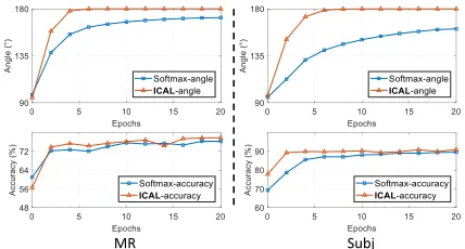
Figure 4: Classification accuracies (%) and inter-class angle (◦) under different epochs on CIFAR-10 dataset.
determine the “dog” example and the margin between class scores of “dog” and “cat” is as large as +8.22. Sim-ilarly, the cat image shown in Fig. 3(b) is also mistakenly classified as “dog” by the existing ResNet. However, by employing our ICAL, the score of “cat” class surpasses that of “dog” by a noticeable margin +9.45. Fig. 3(c) and Fig. 3(d) show similar results. These results further verify the effectiveness of ICAL to help discriminate the examples of similar classes.
• Accuracy vs. Angle In order to see the enhancement of ICAL, Fig. 4 presents the relationship of angle and accuracy under different epochs on CIFAR-10 dataset. Because the CIFAR-10 dataset has ten different cate-gories, and thus we count the smallest angle in the Angular Matrix for each epoch. The general trend is that as the angle increases, the accuracy increases, which further indicates that the angle is positively correlated with the accuracy.
Experiments on Text Datasets
Datasets Description Five popular text classification datasets are utilized for the experiments, which contain
• MRMovie Reviews dataset (Pang and Lee 2005), includ-ing positive and negative emotional polarities.
• CR Customer Reviews (Hu and Liu 2004) of various products (cameras, MP3s, etc.), and the task is to classify positive/negative reviews.
• SubjSubjectivity (Pang and Lee 2004) dataset whose task is to identify a sentence to be subjective or objective.
Table 4: Summary of the text datasets. c: Number of classes. l: Average sentence length. N: Number of sentences. |V|: Vocabulary size. |V pre|: The number of words present in the set of pre-trained word vec-tors. T est: Test mode (CV: 10-fold cross-validation).
Datasets c l N |V| |V pre| T est
MR (Pang and Lee 2005) 2 20 10662 18765 16448 CV
CR (Hu and Liu 2004) 2 19 3775 5340 5046 CV
Subj (Pang and Lee 2004) 2 23 10000 21323 17913 CV
MPQA (Wiebe, Wilson, and Cardie 2005) 2 3 10606 6246 6083 CV
TREC (Socher et al. 2013) 6 10 5952 9592 9125 500
• MPQA Opinion polarity (Wiebe, Wilson, and Cardie 2005) dataset containing news articles from a wide variety of news sources.
• TREC(Socher et al. 2013) question dataset, and the task is to classify a question into one of the six question types.
More details of the above five datasets are listed in Tab. 4.
Baseline Networks To show the adaptability of ICAL to different networks with different classification tasks, we apply ICAL to two types of convolutional neural networks (CNNs) and two types of recurrent neural networks (RNNs) for text classification, which include sentence-level convo-lutional networks (CNN-sen) (Kim 2014), Dynamic Con-volutional Neural Network (DCNN) (Kalchbrenner, Grefen-stette, and Blunsom 2014), Long Short-Term Memory Net-work (LSTM-RNN and Bi-LSTM-RNN) (Tai, Socher, and Manning 2015).
Network Training For the datasets without providing a standard test set, we randomly select 10% of the data as the test set and conduct 10-fold cross-validation for all the compared methods. The reported results are the average of the outputs of 10 independent runs. Following (Kim 2014), training is done through stochastic gradient descent over shuffled mini-batches with the Adadelta (Zeiler 2012).
For the whole datasets, we use the first 40 words of each sentence. And each sentence is zero-padded with less than 40 words. For CNNs, we use: filter windows (h) of 3,4,5 with 150 feature maps for each window, 0.5 for dropout rate (p), and 50 for the min-batch size. In addition, the pre-trained vectors fromword2vec1. For RNNs, the settings are
1
MR Subj
Figure 5: Classification accuracies (%) and inter-class angle (◦) under different epochs on MR and Subj datasets with softmax and ICAL.
kept the same with original networks. The parameterλfor incorporating our ICAL is set toλ= 0.1.
Performance and Analysis For a fair comparison, all the experimental settings are made consistent with the original networks except the developed ICAL.
• Classification AccuracyThe main results are presented in Tab. 3, which clearly show that the accuracy of the original networks can be effectively improved by utilizing the ICAL, so ICAL is critical for both CNNs and RNNs to improve their performance. In particular, on MPQA dataset, the CNN-sen-rand with ICAL (i.e. “CNN-sen-rand+ICAL (ours)”) outperforms the CNN-sen-rand (i.e. “CNN-sen-rand” (Kim 2014)) without ICAL by a margin approximately 2%, which again shows the power of ICAL for text classification.
• Accuracy vs. AngleWe present the curves of accuracy and angle under different epochs on MR and Subj datasets in Fig. 5. The general trend is that as the angle increases, the accuracy increases, which further indicates that ICAL discriminates the examples of similar classes by enlarging the angle between their corresponding class vectors.
• Applicability As shown in Tab. 3, we not only apply ICAL to CNNs, but also to RNNs. In general, it shows that the CNNs and RNNs equipped with ICAL are superior to the original networks in the final performance, which further demonstrates that the ICAL can cover different neural networks on different classification tasks.
Comparison with Large-Margin Loss
Network Settings Liuet al.(Liu et al. 2016) developed a large-margin (L-Softmax) loss function in their work, so it is necessary to compare our ICAL with their loss as well as other typical loss functions. To this end, we apply ICAL to the same network structure as defined in (Liu et al. 2016), and investigate the performance on 10 and CIFAR-100 datasets.
Performance and Analysis In Tab. 5, we list the results produced by different large-margin loss functions and our ICAL. Note that all reported results are directly taken from (Liu et al. 2016) except the results of ICAL. According to
Table 5: Classification accuracies (%) on CIFAR-10 and CIFAR-100 datasets (denoted as “C10”, “C100” for short, respectively). The best result on each dataset is highlighted inbold.
Method C10 C100
R-CNN (Liang and Hu 2015) 91.31 68.25
GenPool (Lee, Gallagher, and Tu 2016) 92.38 67.63
Hinge Loss 90.09 67.10
Softmax 90.95 67.26
L-Softmax (m=2) (Liu et al. 2016) 92.27 70.05
L-Softmax (m=3) (Liu et al. 2016) 92.34 70.13
L-Softmax (m=4) (Liu et al. 2016) 92.42 70.47
ICAL(λ=1.4) (ours) 92.99 70.94
ICAL(λ=1.6) (ours) 93.06 71.09
ICAL(λ=1.8) (ours) 93.04 70.98
ICAL(λ=2.0) (ours) 93.01 70.95
Fig. 2, we select the value of λ from 1.4 to 2.0 with an interval of 0.2.
• Classification Accuracy From Tab. 5, we see that “L-Softmax (m=4) (Liu et al. 2016)” (wheremis an integer. With larger m, the classification margin becomes larger and the learning becomes harder) is the most competitive comparator. However, our “ICAL (λ=1.6) (ours)” with the same structure as “L-Softmax (m=4) (Liu et al. 2016)” can still able to improve its performance on both CIFAR-10 and CIFAR-100 datasets. Therefore, ICAL is more effective than the representative state-of-the-art L-Softmax Loss functions, and the reasons have been explained in the part of related works.
Conclusion
In this paper, we propose a novel general loss function named “Inter-Class Angular Loss” (ICAL) for various rep-resentative convolutional neural networks. By relating the discriminative difficulty of different classes with their angu-lar separability, ICAL is able to enangu-large the angle between the confusing classes, so the distinguishability of networks can be substantially enhanced. The intensive experimental results on both vision and non-vision benchmark datasets confirm that ICAL generates superior performance to the original networks with conventional softmax loss with the consideration of class angular issue. In the future, we plan to apply ICAL to more deep networks to solve more practical problems.
Acknowledgments
References
Deng, J.; Dong, W.; Socher, R.; Li, L.; Li, K.; and Li, F. 2009. Imagenet: a large-scale hierarchical image database. InCVPR.
Gong, C.; Tao, D.; Maybank, S. J.; Liu, W.; Kang, G.; and Yang, J. 2016. Multi-modal curriculum learning for semi-supervised image classification.IEEE Transactions on Image Processing25(7):3249–3260.
Gong, C.; Tao, D.; Liu, W.; Liu, L.; and Yang, J. 2017. Label propagation via teaching-to-learn and learning-to-teach.IEEE Transactions on Neural Networks and Learning Systems28(6):1452–1465.
Hadsell, R.; Chopra, S.; and LeCun, Y. 2006. Dimensional-ity reduction by learning an invariant mapping. InCVPR.
He, K.; Zhang, X.; Ren, S.; and Sun, J. 2016a. Deep residual learning for image recognition. InCVPR.
He, K.; Zhang, X.; Ren, S.; and Sun, J. 2016b. Identity mappings in deep residual networks. InECCV.
Hu, M., and Liu, B. 2004. Mining and summarizing customer reviews. InSIGKDD.
Huang, G.; Liu, Z.; Weinberger, K. Q.; and van der Maaten, L. 2017. Densely connected convolutional networks. In
CVPR.
Kalchbrenner, N.; Grefenstette, E.; and Blunsom, P. 2014. A convolutional neural network for modelling sentences. In
ACL.
Kim, Y. 2014. Convolutional neural networks for sentence classification. InEMNLP.
Krizhevsky, A., and Hinton, G. 2009. Learning multiple layers of features from tiny images. Tech Report.
Krizhevsky, A.; Sutskever, I.; and Hinton, G. E. 2012. Imagenet classification with deep convolutional neural networks. InNIPS.
Lai, S.; Xu, L.; Liu, K.; and Zhao, J. 2015. Recurrent convolutional neural networks for text classification. In
AAAI.
LeCun, Y.; Boser, B.; Denker, J. S.; Henderson, D.; Howard, R. E.; Hubbard, W.; and Jackel, L. D. 1989. Backpropaga-tion applied to handwritten zip code recogniBackpropaga-tion. Neural computation1(4):541–551.
LeCun, Y.; Bottou, L.; Bengio, Y.; and Haffner, P. 1998. Gradient-based learning applied to document recognition.
IEEE86(11):2278–2323.
Lee, C.-Y.; Gallagher, P. W.; and Tu, Z. 2016. Generalizing pooling functions in convolutional neural networks: mixed, gated, and tree. InAISTATS.
Li, X.; Yang, F.; Chen, L.; and Cai, H. 2016. Saliency transfer: an example-based method for salient object detection. InIJCAI.
Liang, M., and Hu, X. 2015. Recurrent convolutional neural network for object recognition. InCVPR.
Liu, W.; Wen, Y.; Yu, Z.; and Yang, M. 2016. Large-margin softmax loss for convolutional neural networks. InICML.
Liu, P.; Qiu, X.; and Huang, X. 2016. Recurrent neural network for text classification with multi-task learning. In
IJCAI.
Pang, B., and Lee, L. 2004. A sentimental education: sentiment analysis using subjectivity summarization based on minimum cuts. InACL.
Pang, B., and Lee, L. 2005. Seeing stars: exploiting class relationships for sentiment categorization with respect to rating scales. InACL.
Schroff, F.; Kalenichenko, D.; and Philbin, J. 2015. Facenet: a unified embedding for face recognition and clustering. In
CVPR.
Simonyan, K., and Zisserman, A. 2015. Very deep convolutional networks for large-scale image recognition. In
ICLR.
Socher, R.; Perelygin, A.; Wu, J. Y.; Chuang, J.; Manning, C. D.; Ng, A. Y.; Potts, C.; et al. 2013. Recursive deep models for semantic compositionality over a sentiment treebank. InEMNLP.
Srivastava, R. K.; Greff, K.; and Schmidhuber, J. 2015. Highway networks. InICML.
Szegedy, C.; Liu, W.; Jia, Y.; Sermanet, P.; Reed, S.; Anguelov, D.; Erhan, D.; Vanhoucke, V.; and Rabinovich, A. 2015. Going deeper with convolutions. InCVPR. Szegedy, C.; Vanhoucke, V.; Ioffe, S.; Shlens, J.; and Wojna, Z. 2016. Rethinking the inception architecture for computer vision. InCVPR.
Szegedy, C.; Ioffe, S.; Vanhoucke, V.; and Alemi, A. A. 2017. Inception-v4, inception-resnet and the impact of residual connections on learning. InAAAI.
Tai, K.; Socher, R.; and Manning, C. D. 2015. Improved semantic representations from tree-structured long short-term memory networks. InACL.
Wang, J.; Wang, Z.; Zhang, D.; and Yan, J. 2017. Combining knowledge with deep convolutional neural networks for short text classification. InIJCAI.
Wen, Y.; Zhang, K.; Li, Z.; and Qiao, Y. 2016. A discriminative feature learning approach for deep face recognition. InECCV.
Wiebe, J.; Wilson, T.; and Cardie, C. 2005. Annotating expressions of opinions and emotions in language. InLRE. Xiao, H.; Rasul, K.; and Vollgraf, R. 2017. Fashion-mnist: a novel image dataset for benchmarking machine learning algorithms.arXiv preprint arXiv:1708.07747.
Xie, S.; Girshick, R.; Dollar, P.; Tu, Z.; and He, K. 2017. Aggregated residual transformations for deep neural networks. InCVPR.
Zagoruyko, S., and Komodakis, N. 2016. Wide residual networks. InBMVC.
Zeiler, M. D. 2012. Adadelta: an adaptive learning rate method.arXiv preprint arXiv:1212.5701.