The Thirty-Third AAAI Conference on Artificial Intelligence (AAAI-19)
Probabilistic Model Checking of Robots Deployed in Extreme Environments
Xingyu Zhao,
1Valentin Robu,
1,2David Flynn,
1Fateme Dinmohammadi,
1Michael Fisher,
3Matt Webster
31School of Engineering & Physical Sciences, Heriot-Watt University, Edinburgh EH14 4AS, U.K. 2Center for Collective Intelligence, Massachusetts Institute of Technology, Cambridge MA 02139, U.S.
3Department of Computer Science, University of Liverpool, Liverpool L69 3BX, U.K.
Email:{xingyu.zhao, v.robu, d.flynn, f.dinmohammadi}@hw.ac.uk,{mfisher, matt}@liverpool.ac.uk
Abstract
Robots are increasingly used to carry out critical missions in extreme environments that are hazardous for humans. This re-quires a high degree of operational autonomy under uncertain conditions, and poses new challenges for assuring the robot’s safety and reliability. In this paper, we develop a frame-work for probabilistic model checking on a layered Markov model to verify the safety and reliability requirements of such robots, both at pre-mission stage and during runtime. Two novel estimators based on conservative Bayesian inference and imprecise probability model with sets of priors are intro-duced to learn the unknown transition parameters from oper-ational data. We demonstrate our approach using data from a real-world deployment of unmanned underwater vehicles in extreme environments.
1
Introduction
Extreme environments, as a term used by UK EPSRC1 to
denote environments that are remote and hazardous for hu-mans, are one of the most promising application areas in which robots can be deployed to carry out a task, such as in-specting oil and gas equipment, maintaining offshore wind turbines or monitoring nuclear reactors. Interaction with hu-man operators is often infeasible in such remote environ-ments, so autonomy becomes a key requirement, meaning robots have to learn to adapt when performing tasks in changing and unexpected circumstances (Lane et al. 2016).
However, unforeseen behaviour of a robot could result ei-ther in failure of its own mission or even undermine the in-tegrity of the asset being inspected or repaired – with po-tentially catastrophic consequences, e.g. accidental punc-ture of subsea pipelines. The robots themselves are high-value assets, whose loss or damage may be very costly. Moreover, there are increasing demands on regulating au-tonomous robots to build public trust in their use. Yet, the analysis of safety and reliability for autonomous robots poses a significant challenge due to the inevitable uncertain-ties in a mission. Potential sources of risk range from failures of sensors or hardware, to built-in algorithms making poor choices in a stochastic environment. Key industrial foresight reviews (Lane et al. 2016) outline a vision ofself-certifying
Copyright c2019, Association for the Advancement of Artificial Intelligence (www.aaai.org). All rights reserved.
1
https://epsrc.ukri.org/files/funding/calls/2017/raihubs/
robotic systems, i.e. systems that continuously monitor their current and predicted performance and assess it within a predefined certification framework (Robu, Flynn, and Lane 2018; Fisher et al. 2018).
Probabilistic model checking (PMC) (Kwiatkowska, Nor-man, and Parker 2018) has been successfully used to anal-yse quantitative properties of systems across a variety of application domains, including robotic systems (Luckcuck et al. 2018). This involves the construction of a probabilis-tic model, commonly using Discrete Time Markov Chain (DTMC), Continuous Time Markov Chain (CTMC) and Markov Decision Process (MDP) when considering non-deterministic actions, that formally represents the behaviour of a system over time. The properties of interest are nor-mally specified in Linear Temporal Logic (LTL) or Proba-bilistic Computational Tree Logic (PCTL), then systematic exploration and analysis is performed to check if a claimed property holds.
One inherent problem for most (if not all) formal verifi-cation techniques is that the verifiverifi-cation assumes the formal model (e.g. DTMC) accurately reflects the actual behaviour of the real-world system (Calinescu et al. 2016). Compar-ing to conventional systems - for which we might argue the formal model is fairly accurate – it becomes a tougher is-sue for systems in changing, unexpected environments and with autonomous features. To handle the issue, the run-time verification idea was proposed (Epifani et al. 2009; Calinescu et al. 2012) by keeping the formal model alive and continuously updated when seeing new data at runtime. In this paper, we propose a tailored PMC framework for verifying safety-critical robots working in extreme environ-ments. Firstly, we formalise how the robot works as a lay-ered and parametric DTMC (transition probabilities are un-known parameters), then feed two Bayesian estimators for different types of parameters with operational data. For each mission, safety and reliability properties are verified at both:
Pre-mission, based on the best knowledge from previous similar missions, lab-simulations and experts, which pro-vides assurance before the robot undertaking a mission.
of the robot’s front-end planning engine. This follows the “defence in depth” design paradigm for safety critical sys-tems, by providing an extra and diverse layer of protection.
To achieve these, we identify two types of transition pa-rameters and introduce two novel Bayesian estimators as:
A. Catastrophic failure related parameters, which repre-sent the probability of seeing a catastrophic failure when the robot is in an unsafe state. In practice, we cannot observe sufficient data of catastrophic failures to provide good esti-mations, since even if we do observe any, we normally will redesign/update the robot making the failure data obsolete. So effectively, for these model parameters, we will only col-lectfailure-freedata that lead to very optimistic estimations by existing Bayesian estimators. To avoid underestimating the chances of catastrophic failure, our claim is inference in such settings has to be carried out in a conservativeway. The conservative Bayesian inference (CBI) method (Bishop et al. 2011; Strigini and Povyakalo 2013; Zhao et al. 2015; 2017) was developed for safety-critical software to answer the question what can be claimed rigorously about the relia-bility when seeing failure-free runs. To our knowledge, our work is the first to develop a CBI estimator for catastrophic failure parameters in robotics.
B. Non-catastrophic failure related parameters, which represent the transitions among normal, unsafe and non-catastrophic states, thus sufficient data can be collected as more missions are conducted. Bayesian methods yielding point estimates, e.g. (Epifani et al. 2009; Calinescu et al. 2014), are affected by unquantified estimation errors which will be propagated and compounded in the verification in ways that are unknown but likely to be significant, as high-lighted in (Calinescu et al. 2016). Here we introduce an im-precise probability model withsets of priors(Walter and Au-gustin 2009; Walter, Aslett, and Coolen 2017) to (i) get up-per and lower bounds on the posterior estimates whose range measures the estimation errors; (ii) allow modelling imper-fect prior knowledge/data from experts/lab-simulations in a flexible way; and (iii) detectprior-data conflict (Evans and Moshonov 2006) when observe surprising data in a mission to provide protection from the robot’s epistemic limits.
We illustrate our new method with an example of an un-manned underwater vehicle (UUV) in the context of a valve turning scenario from the PANDORA2 project which
cre-ated UUVs that keep going under extreme uncertainty. Next, we present the necessary background concepts. Two new Bayesian estimators are described in Section 3; Section 4 describes the new framework with an illustrative example. Section 5 summarises the related work. Contributions, limi-tations and future work are concluded in Section 6.
2
Preliminaries
2.1
DTMC and PCTL
Discrete Time Markov Chain (DTMC) is a widely-used model for formalising stochastic systems. From the verifi-cation point of view, DTMC can serve as a secondary pro-tection modelgivenan optimal policy (specifying a proce-dure for autonomous action selection). For instance, if the
2
http://persistentautonomy.com/?p=1436
primary planner synthesises an optimal policy via MDP and reinforcement learning (Pathak, Pulina, and Tacchella 2018; Pathak et al. 2013), then given the optimal policy, we obtain aninduced DTMC(Puterman 2014) which can be revised to emphasise the safety and reliability aspects by, e.g. adding more transitions to states representing hazards.
Definition 1. A DTMC is a tuple(S, s1,P, L), where:
• Sis a (finite) set of states; ands1∈Sis an initial state;
• P:S×S→[0,1]is a probabilistic transition matrix such thatP
s0∈SP(s, s0) = 1for alls∈S;
• L : S → 2AP is a labelling function assigning to each state a set of atomic propositions from a setAP.
We use the notationpij =P(si, sj), andi, jare integers in [1, k] by assuming there arek states in total. Given an optimal probabilistic3policy, the transition probability of the
induced DTMC is defined as the total probability of:
pij =X a∈A
πa(si)·P r(sj |si, a) (1)
whereπa(si)is the probability of executing actionain state si according to policyπ andP r(sj|si, a)is the probabil-ity that sj is the next state when action a is executed in
statesi. In this paper, we assume the optimal policyπ, i.e.
πa(si), is given by a separate planner andP r(sj|si, a)will be Bayesian updated via operational data.
The safety and reliability properties to be checked can be specified in Probabilistic Computation Tree Logic (PCTL).
Definition 2.AP is a set of atomic propositions andap∈ AP, p ∈[0,1], t∈Nand./∈ {<,≤, >,≥}. The syntax of
PCTL is defined bystate formulaeΦandpath formulaeΨ.
Φ ::=true|ap|Φ∧Φ| ¬Φ| P./p(Ψ)
Ψ ::=XΦ|ΦU≤tΦ
where the temporal operatorXis calledNextandUis called
Until. State formulaeΦis evaluated to be either true or false in each state. Satisfaction relations for a statesare defined:
s|=true , s|=ap iff ap∈L(s) s|=¬Φ iff s6|= Φ
s|= Φ1∧Φ2 iff s|= Φ1ands|= Φ2
s|=P./p(Ψ) iff P r(s|= Ψ)./ p
P r(s|= Ψ)./ pis the probability of the set of paths start-ing insand satisfyingΨ. Given a pathψ, if denote itsi-th state asψ[i]andψ[0]is the initial state. Then the satisfaction relation for a path formula for a pathψis defined as:
ψ|=XΦ iff ψ[1]|= Φ
ψ|= Φ1U≤tΦ2 iff ∃0≤j≤t
(ψ[j]|= Φ2∧(∀0≤k < j ψ[k]|= Φ1))
It is worth mentioning that both DTMC and PCTL can be augmented with rewards/costs, cf. (Filieri and Tambur-relli 2013), which can be used to model, e.g. the energy/time
3
consumption of the robot in a mission. Our approach is also compatible for those properties which we omit in this paper. By formalising the robot and its required properties in DTMC and PCTL respectively, the verification focus shifts to the checking ofreachabilityin a DTMC. In other words, PCTL expresses the constraints that must be satisfied con-cerning the probability, starting from the initial state, of reaching some states being labelled as, e.g. unsafe, failure or success. We use the tool PRISM (Kwiatkowska, Norman, and Parker 2011) which employs symbolic model checking algorithm to calculate the actual probability that a path for-mulae is satisfied (by extending the PCTL definition with P=?(Ψ)), then comparing with a required bound if given.
2.2
Parametric model checking
PMC based on DTMC normally assumes the transition prob-abilities are known as constants which can be estimated from existing data and experts at design-time, or through system runtime monitoring. However, this traditional technique may not be suitable for runtime analysis in terms of the exces-sive time and power consumption, especially for robots. The idea ofparametricmodel checking (ParaMC), proposed by (Daws 2005), provides an efficient solution (Filieri, Ghezzi, and Tamburrelli 2011). As shown by (Jansen et al. 2014), modern tools can solve parametric DTMCs with thousands of states and transitions using reasonable computing re-sources, beyond the required capability of our methods here. ParaMC can analyse DTMC whose transition probabili-ties are specified as functions over a set of parameters, e.g. Equation (1). The result is then given as a closed-form ra-tional function of the parameters which brings two advan-tages: (i) The verification can be divided into two steps. The computationally expensive symbolic analysis can be done at pre-mission stage when time and power constraints are not strong; then, during the mission, only substitutions are needed to replace the parameters in the closed-form expres-sion with actual values learnt at runtime; (ii) Monotonic-ity analysis of the parameters can be easily done via the closed-form expression. Since, instead of point estimates, our new Bayesian estimator provides bounds for the parame-ters, thus monotonicity analysis is necessary to obtain mean-ingful bounds for the verification results.
3
Estimates for DTMC transition parameters
3.1
A fundamental Bayesian estimator
In a DTMC, given a current statei, the transition to a next state follows acategorical distribution. Due to the Markov property, i.e. the choice of a next state only depends on the current one, the categorical distributions for each state areindependent. Hence, as we observe repeated transitions from the statei, the repeated categorical process follows a
multinomial distribution. Now the problem is reduced to the
localised learning ofk independent multinomial distribu-tion, wherekis the number of states in the DTMC. From a Bayesian inference perspective, the posterior estimation requires a statistical model (the likelihood function) and a prior distribution. Note a complete description of Bayesian inference is beyond the scope of this paper.
For thei-th row ofP, if we observe the data of transition number from stateitoj asnij, andni =Pkj=1nij is the total number of outgoing transitions from statei, then the likelihood function is (by omitting the combinatorial factor which will be cancelled in the Bayesian formula):
P r(data|pi1, ..., pik) = k Y j=1
pnij
ij (2)
The method in (Epifani et al. 2009) uses a Dirichlet dis-tribution as priors for a giveni-th row ofP:
(pi1, ..., pik)∼Dir(n (0)
i p
(0)
i1 , ..., n (0)
i p
(0)
ik ) (3)
wheren(0)i p(0)i1, ..., n(0)i p(0)ik are thecanonical parameters
of the Dirichlet.p(0)ij is the prior expectation for the transition
probabilitypij, and largern
(0)
i leads to more concentrated
probability measure aroundp(0)ij . Thus,n(0)i are quantifying
the strength of beliefs in the priorp(0)ij , or a “pseudo-count” which can be interpreted as the size of an imaginary sample that gives the prior estimation (Walter and Augustin 2009).
Then applying the Bayes rule, and thanks to both the con-jugacy (with the multinomial likelihood function) and the canonical form, the posterior with updated parameters are:
n(ni)
i =n
(0)
i +ni (4)
p(ni)
ij = n(0)i
n(0)i +ni
·p(0)ij + ni n(0)i +ni
·nij ni
(5)
Note, the upper index(0) is used to identify the prior
pa-rameters, in contrast, the(ni) denotes the posterior
param-eters after observingni outgoing transitions from the state i. As Equation (5) shows, after seeingnijout ofnias data, the posteriorp(ni)
ij is aweightedsum of two terms: the prior
estimate ofp(0)ij and thenij/niwhich is the frequency of the relevant transition in the data. The weights are proportional to then(0)i (the “pseudo-count” of prior simple size) andni
(the “actual-count” of data sample size). Smallern(0)i rep-resents lower confidence in the priors and the runtime data will dominate the posteriors. Whenn(0)i '0, (5) reduces to the Maximum Likelihood Estimation (Epifani et al. 2009).
3.2
A Bayesian estimator using sets of priors
prior knowledge by eliciting bounds of the prior parameters, and also resulting bounds for the posteriors whose range measures the estimation errors. Also importantly, it is sen-sitive to detect theprior-data conflict, i.e. conflicts between prior assumptions and observed data (Evans and Moshonov 2006), which is useful to alter dangerous situations and will be discussed later.
To be exact, instead of a single value, we elicit an interval for each prior parameters in (3) and denote these as:
n(0)i ∈hni(0), ni(0)i , p(0)ij ∈hpij(0), pij(0)i
Then as proved in (Walter and Augustin 2009), the lower and upper bounds for the posteriors of interestp(ni)
ij are:
pij(ni)=
ni(0)pij(0)+nij
ni(0)+ni if
nij
ni ≥pij (0)
ni(0)pij(0)+nij
ni(0)+ni if
nij
ni < pij
(0) (6)
pij(ni)=
ni(0)pij(0)+nij
ni(0)+ni if
nij
ni ≤pij (0)
ni(0)pij(0)+nij
ni(0)+ni if
nij
ni > pij
(0) (7)
When nij
ni ∈/
h
pij(0), pij(0)i, i.e. the prior-data conflict
is at hand, the posterior intervalhpij(ni), pij(ni) i
becomes wider, meaning we areeven less certainabout the posterior estimation comparing to the priors. This is a new property comparing to other imprecise probability models in which the range of the posterior interval will always, regardless of the prior-data conflict, decrease (i.e. converge to the ob-served data) as the sample size increases.
3.3
Conservative Bayesian inference
Catastrophic failures are modelled in our new framework by imposing transitions from unsafe states to catastrophic failures of different modes, e.g. the parameter x in Fig.1 as an instance. The “true unknown” values of these transi-tion parameters may lie in very small orders of magnitude, say10−5 →10−9, as a result of rigorous development
pro-cess and safety-critical designs. This poses a great challenge for the estimation of such smaller failure rates in terms of that infeasible amount of statistical testing or operational time is required to observe sufficient failure data (Littlewood and Strigini 1993). More practically, even if we did observe any catastrophic failures, we normally will redesign/update the robots, which makes the failure data obsolete. So ef-fectively, we will only collectcatastrophic-failure-freedata. Such “good news” would increase our confidence that the robot has a smaller chance to cause catastrophic failures, hence our claim is such inference has to be done in a con-servativeway. The conservative Bayesian inference (CBI) method (Bishop et al. 2011; Strigini and Povyakalo 2013; Zhao et al. 2015; 2017) was developed for safety-critical software to answer what can be claimed rigorously about the reliability when seeing failure-free runs. Here we introduce CBI as our Bayesian estimator for the catastrophic failure related parameters. Note, we only present the more practi-cal case of seeing no catastrophic failures in this paper. The essential CBI can be extended to model very scarce failures.
In a given unsafe statei, as discussed above, the outgoing transitions follow a multinomial distribution, somarginally, the number of transitions to the catastrophic failure state, saynij, is a binomial one,nij ∼Bin(ni, x)wherexis the transition probability and ni is the total number of
outgo-ing transitions from statei. Then the likelihood function for the data of no catastrophic failure observed, i.e. nij = 0,
is:P r(data|x) = (1−x)ni. So if we have a prior
distribu-tion forx, sayf(x), by Bayes rule we know the posterior expectation is:
E(x|data) = R1
0 x(1−x)
nif(x)dx
R1
0(1−x)nif(x)dx
(8)
Conventionally, starting from Equation (8), we assign a parametric family forf(x), e.g. a conjugate Beta in this case, or like the Dirichlet-Multinomial case in Section 3.1. How-ever, the use of conjugacy is based on the assumption that the practical situations we are dealing with have large quan-tities of failure data, in which the dominant contribution to posterior belief via Bayes Theorem comes from the likeli-hood function, i.e. situations in which “the data can speak for themselves”. We do not have this luxury for safety-critical systems with very limited or no failure data, so any use of a particular parametric family forf(x)is questionable.
Instead of assuming acompleteprior distribution that fol-lows a parametric family, the assessors are more likely to have (or be able to justify) some very limitedpartialprior knowledge, e.g. two possible scenarios: (i) “I am 80% con-fident the robot will not have any catastrophic failure in this unsafe state” is a confidence in its catastrophic-failure-freeness, i.e. P r(x = 0) = 0.8. See (Littlewood and Rushby 2012; Strigini and Povyakalo 2013) for the argu-ments of such partial prior knowledge; (ii) “I am 90% confi-dent the probability of seeing a catastrophic failure from this unsafe state is smaller than 0.001” is a confidence bound on a given probability of seeing catastrophic failure, i.e.
P r(x≤0.001) = 0.9. Such partial prior knowledge could be supported by, e.g. when evidence is presented showing the system is strictly developed against IEC61508 SIL34.
In the above scenarios, the elicited partial prior knowledge is far from a complete prior distribution. Rather, if treat the partial priors asconstraintson a distribution, then there must be aninfinite set of prior distributions satisfying the prior constraints. Note, this set of priors is different from the one in Section 3.2 which still assumes a parametric family (i.e. Dirichlet). Now the problem reduces to find themost conser-vativeprior distribution (in the sense of giving a maximum posterior expected transition probability) in the infinite set of priors satisfying the elicited prior constraints.
For example, as the first scenario, the assessor only has a
θconfidence in its catastrophic-failure-freeness:
P r(x= 0) =θ (9)
As proved in (Strigini and Povyakalo 2013), to maximise (8), the correspondingf(x), that subjects to the constraint (9), is a two-point one with probability mass at P r(x =
4
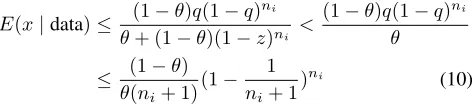
0) = θ andP r(x =q) = 1−θ, whereqis an optimisa-tion point that can be obtained numerically. Thus, by such two-pointf(x), Equation (8) can be further bounded by:
E(x|data)≤ (1−θ)q(1−q) ni
θ+ (1−θ)(1−z)ni <
(1−θ)q(1−q)ni
θ
≤ (1−θ) θ(ni+ 1)(1−
1 ni+ 1)
ni (10)
Note the last step above is because thatq(1−q)ni reaches
its maximum whenq= 1/(ni+ 1).
Depending on the particular form of partial prior knowl-edge elicited, the worst-case priors varies, so does the pos-teriors. For cases of other forms of partial prior knowledge, see (Bishop et al. 2011; Zhao et al. 2015; 2017).
To summarise, in this section, we present two advanced Bayesian estimators for the two types of transition param-eters. Mixed use of incorrect estimators will lead to either “too conservative to be useful results” or “continuous prior-data conflict”, which we omit here due to the page limit.
4
The framework with an UUV example
4.1
The running example
We use an underwater search and valve turning mission in which a UUV equipped with electrical manipulators, stereo cameras, a specifically designed end-effector which had a camera in-hand with force and torque sensors to (i) locate a valve panel among different locations; and (ii) modify the valve handles to achieve different panel configurations. Pos-sible disturbances are, e.g. muddy water, strong currents, blocked valves and panel occlusion. We formalise a single valve operation as an instance of the DTMC in Fig. 1 which has been simplified with only 6 states, whilst more realis-tic formal models, e.g. with more states and transitions as shown as the dotted shapes in the figure, can be obtained in our proposed generic way as follows.
The DTMC in Fig. 1 has 3 layers. The normal operation and safe states are modelled in the first layer, in which each state can transit into one or more unsafe states with some probabilities, e.g. in theS1 state of searching valve panel, the UUV may encounter a region of muddy water leading to the unsafe low visibility stateS4. We group all the un-safe states in the middle layer which can either transit back to the normal operations or cause various modes of failures, including catastrophic ones, in the bottom layer, e.g. the pro-peller has a higher risk of malfunction when the UUV is in a muddy water. We believe the structure of a realistic DTMC can be built in a generic way that the top layer can be de-rived from the original policy-making model, e.g. MDP and reinforce learning as in (Pathak, Pulina, and Tacchella 2018; Pathak et al. 2013), and the bottom two layers can be ob-tained from traditional safety and reliability analysis based on expert knowledge like Failure Mode, Mechanism and Ef-fect Analysis (FMMEA) and Fault Tree Analysis (FTA).
Practically, most of the transition probabilities in the for-mal Markov model can be argued as known constants, e.g. by prognostics on the remaining useful life of key compo-nents (Romain et al. 2017), leaving only a few transition
Figure 1: A layered DTMC modelling an UUV in a valve turning mission. The dotted shapes illustrate possible exten-sions to make the simplified example more realistic.
probabilities as unknown parameters, e.g. thexandyin Fig. 1 (thus a parametric DTMC), which will be Bayesian esti-mated at runtime with collected data.
Fig. 1 is also an induced DTMC, since we assume the
givenoptimal policy is a probabilistic one forS1, e.g. withγ
probability to do speed-1 and(1−γ)probability to do speed-2, whereγis learnt by a separate primary planner. Then the induced transition probability fromS1toS2is a function of
a1, a2as given by Equation (1):a(a1, a2) =γa1+(1−γ)a2
wherea1anda2are the probabilities of transiting fromS1to
S2with autonomous speed-1 and speed-2 respectively. Sim-ilarly forb(b1, b2). ForS4, we assume a deterministic policy
(e.g. always do safe mode speed in low visibility), thus the outgoing transition probabilities are single parameters.
We are interested in 4 requirements: R1: What is the probability of completing anextmission? R2:What is the probability of seeing catastrophic failures in anextmission?
R3:What is the probability of completingthismission?R4:
What is the probability of seeing catastrophic failures inthis
mission? The R1 and R2 will be analysed at the pre-mission stage, whose PCTL with the initial state specified asS1are:
P=?[true U(s= 3)] , P=?[true U(s= 6)]
Whilst, R3 and R4 will be verified at runtime. Their PCTL are same as above but with different specified initial states.
4.2
The framework and simulated experiments
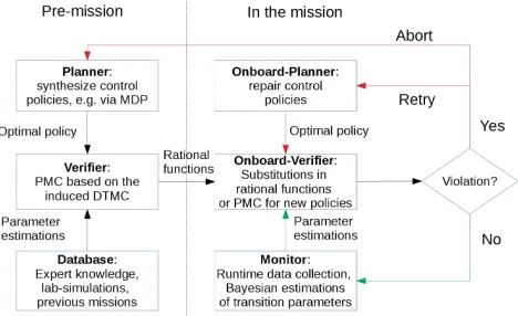
As shown in Fig. 2, our framework has two stages:
recorded and also reused by the on-board verifier to speed up the verification at runtime. Monotonicity analysis for each parameter in the rational functions is necessary due to the use of bounds for each transition parameter. Data analysis of experts’ knowledge, lab-simulations and previous similar missions is performed to form prior knowledge required by the two Bayesian estimators. Finally, by substituting param-eters in the rational functions with the prior estimates, pre-mission verification results are obtained, which represents our best efforts of assurance before launching the robot.
In mission (runtime), a monitor collects new data and does Bayesian estimates on the transition parameters. The on-board verifier checks if any required properties are being vi-olated at runtime based on the ParaMC results at pre-mission stage. When any violation presents, actions like abort or in-stantly restart the mission (with a repaired policy) can be taken, whose implementation is beyond the scope of this pa-per. Otherwise, the UUV will continue and keep monitoring and verifying until the mission is complete.
Figure 2: Overview of the verification framework.
We demonstrate and evaluate our framework by simulated experiments based on the UUV example of Fig. 1. First, to simulate and collect data of both previous missions and the current one for the pmission and runtime verifications re-spectively, we use the PRISM simulation module by assum-ing thetrue unknowntransitions probabilities in Fig. 1 are:
a1 = 0.05, a2 = 0.03, b1 = 0.2, b2 = 0.1, x = 10−5, y =
0.001, v = 0.3, w = 0.01. For the optimal policy of state 1, we assign a random number in [2540,3540] 5 for γ in each simulated mission to mimic the practical case of changing policies. Then, it results in 49 previous missions and a 50-th as the current one6 which explicitly usingγ = 0.75as the
optimal probabilistic policy of state 1.
At the pre-mission stage, given the data of previous 49 missions (e.g. 1566 outgoing transitions fromS1 with the action of speed-1, in which 1180 loops inS1, 85 toS2and 301 toS4), together with the prior knowledge in Table 1, the posteriors by our Bayesian estimators are also listed there.
5
All assumed values of the parameters in the simulation refer to the information provided by the PANDORA project.
6
Without loss of generality, we choose a 50-th mission with relatively more transitions (522 to be exact) for a better illustration.
Next, given γ = 0.75and using the ParaMC engine of PRISM, we obtain closed-form results for R1 and R2 (also R3 and R4 with different initial states for the use at runtime) as rational functions whose monotonicity can be easily anal-ysed with respect to the 8 transition parameters. Then we obtain the pre-mission verification results:
R1∈[0.857,0.961], R2∈
7.96×10−4,1.55×10−3
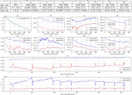
In the current 50-th mission, the posteriors of the 8 tran-sition parameters in Table 1 are in turn used as priors for the runtime Bayesian updates. The real-time estimates at each discrete time step of the transitions are plotted in (a)-(h) of Fig. 3, correspondingly R3 and R4 are plotted in (i) and (j).
As shown in the (a) of Fig. 3, the CBI estimation forx de-creases along with the execution of the robot without catas-trophic failures. For non-catascatas-trophic failure related param-eters of (b)-(h), instead of using CBI to obtain a conservative point estimation, we plot both upper and lower bounds via Bayesian inference with sets of priors. Basically for each of these parameters, we first observe a divergence trend of the two bounds which then start to converge as more data is collected. Indeed, at the beginning of a mission, due to the sparse data collected, the prior-data conflict phenomenon is normal and foreseeable (e.g. 3 heads out of 3 tosses of a fair coin is conflicting our prior belief in its fairness). Such conflict is reflected by a wider bounded (i.e. less certain) estimation for each parameter and then propagated to the overall verification results.
For instance, verifications on both R3 and R4 become less and less certain in the first 100 steps, partly due to the prior-data conflict ofa1. Then, the 101-th step is a transition from
S1 toS2 with speed-1 action, which not only provides a new estimate ofa1 but also resolves the prior-data conflict
to some extent, leading to tighter bounds fora1, R3 and R4.
As more runtime data is observed, the general trend for each pair of bounds in Fig. 3 starts to converge, meaning a more certain verification result. Note, both R3 and R4 highly depend on which state the UUV is currently in, so the obvi-ous “bumps” in the plot for R3 are because the UUV is in
S2 which certainly has a relatively higher chance to com-plete the mission. Similarly for the bumps in the plot of R4. The above example is an ideal case in the sense that the new learning agrees with what it learnt before, i.e. all the 50 missions are simulated based on an MDP with the same tran-sition probabilities, like the probability of transiting back to the normal stateS1from the low visibility stateS4is con-stantly assumed asv = 0.3for all 50 missions. For excep-tional cases, e.g. there is a large body of muddy water im-plyingv = 0.8, our method will detect them as prior-data conflict through the whole mission, thus a continuous diver-gence of the bounds of related transition parameters will be observed, so consequently does an overall divergence of the verification results R3 and R4. We label this exceptional case as “known unknowns” in the sense that the new unknown (e.g.v = 0.8) is learnt in an informed way such that we know how much contradict it is to our prior knowledge, thus leading a less certain (i.e. wider bounds) new estimation.
Table 1: Prior knowledge and posterior estimations for the transition parameters given the data of 49 previous missions.
x y v w a1 b1 a2 b2
pse. cou. N/A [100,300] [100,300] [100,300] [100,300] [100,300] [50,100] [50,100]
pri. est. θ= 0.9 [0.001,0.01] [0.1,0.4] [0.001,0.01] [0.01,0.1] [0.1,0.5] [0.01,0.1] [0.1,0.5]
post. est. 3.2e-5 [0.0014,0.0032] [0.27,0.33] [0.0097,0.012] [0.047,0.062] [0.18,0.24] [0.03,0.04] [0.09,0.16]
Figure 3: Runtime Bayesian estimations for the 8 transition parameters (a)-(h) and verification results for R3 (i) and R4 (j).
which state it is in andwithout knowing this fact. For ex-ample, the UUV now is in a muddy water (i.e.S4), but the sensor fails to detect this unsafe state so that the UUV be-lieves it is still in the normal stateS1. As a consequence, the UUV does a wrong action of either speed-1 or speed-2 (i.e. the probabilistic policy inS1) in the unsafe stateS4instead of the safe speed (i.e. the deterministic policy forS4). Our method is also able to alert such dangerous case by detect-ing prior-data conflict phenomenon that happens simultane-ouslyfor many parameters. Because, in the example above, although the UUV isactuallyinS4, it willexperience con-stant loops in S1 without transiting to neither S4 (as the sensors fail to detect the abnormal states) norS2(as wrong actions are taken, assuming going fast in a muddy water will never detect the valves). Consequentially, prior-data conflict happens simultaneously for alla1, a2, b1, b2parameters.
More examples for the exceptional cases of “known un-knowns” and “unknown unun-knowns” will be discussed in fu-ture due to the page limits here. We believe, detecting the prior-data conflict effect during the mission can assure
pro-tection against from faulty knowledge (i.e. epistemic limits) of the robot about its own state of health and environments.
5
Related work
How should autonomous systems be verified is a new chal-lenging question along with their increasing applications (Fisher, Dennis, and Webster 2013). Formal methods must be integrated in order to develop, verify and provide certi-fication evidence for large-scale and complex autonomous systems like robots (Farrell, Luckcuck, and Fisher 2018).
analysed by PMC. In (Norman, Parker, and Zou 2017; Pathak, Pulina, and Tacchella 2018), PMC is used to verify the control policies of robots in partially unknown environ-ments. In a hostile environment, the movements of adver-saries are modelled probabilistically in (Cizelj et al. 2011). The reliability and performance of UUVs is guaranteed by PMC in (Gerasimou, Calinescu, and Banks 2014).
Although runtime PMC is effective for assuring the qual-ity of service-based systems (Calinescu et al. 2011) and self-adaptive systems (Calinescu et al. 2012; Filieri and Tam-burrelli 2013), there is little research on runtime PMC for robots. In the UUV domain, the first work of runtime PMC is credited to (Gerasimou, Calinescu, and Banks 2014). How-ever, it focuses on improving the scalability of runtime PMC by using software engineering techniques, which is also ap-plicable to our work here that focuses on developing new methods of learning model parameters.
One of the initial methods to learn the transition prob-abilities of DTMC is in (Epifani et al. 2009), which later has been retrofitted for CTMC (Filieri, Ghezzi, and Tam-burrelli 2012) and extended with ageing factors of collected data to accurately estimate time-varying transition probabil-ities (Calinescu et al. 2014). To reduce the noise and provide smooth estimates, a lightweight adaptive filter is proposed in (Filieri, Grunske, and Leva 2015). Whilst, above mentioned approaches yield point estimations, these can be affected by unquantified and potentially significant errors. The work in (Calinescu et al. 2016) is the first to synthesise bounds for unknown transition parameters. However, it is based on the theory of simultaneous confidence intervals, which is funda-mentally different to the Bayesian approach presented here which has the distinct advantage of being able to embed var-ious forms of prior knowledge.
6
Conclusions & future work
In this paper, we present a new framework to utilise PMC to assess the safety and reliability of robots at both pre-mission stage and runtime. Our main contributions are:
1. CBI is introduced with new closed-form results as a novel estimator for catastrophic failure related parameters.
2. Imprecise probability with sets of priors is introduced as another novel estimator for transition parameters. It al-lows to not only quantify the estimation errors and flex-ibly model imperfect prior knowledge, but also detect prior-data conflict to alter various dangerous situations.
3. A generic way is discussed to structure Markov models into layers to emphasise the system safety and reliability.
4. A real-word application of UUVs has been formalised which can be extended and reused for future research.
For illustration purpose, we demonstrate our methods with a stylised example which can be easily extended in our proposed generic way without changing the main conclu-sions, e.g. by considering the geographical waypoints in the top layer of the DTMC or listing complete failure modes in the bottom layer. The practicality of our new approach needs to be further evaluated with more case studies. We see potential issues like (i) insufficient safety analysis in
FTA/FMMEA to generate sound DTMC in the bottom two layers; and (ii) unnecessarily complex DTMC model with too many unknown transition parameters which require too much prior knowledge from experts and too much data to be collected at runtime that burdens the on-board sensors.
We plan to exploit more use of prior-data conflict and also
strong prior-data agreement (Walter and Coolen 2016) to reflect the robot’s epistemic limitations. Requirements to be verified for a robot should come from a higher level, e.g. when a robot is part of the Prognostics and Health Man-agement (PHM) system, a PHM level PMC can be done in future to answer what to certify a robot. We also plan to pro-pose a lightweight on-board re-planner based on an MDP with the up-to-date bounded transition parameters.
7
Acknowledgements
This work was supported by the UK EPSRC, through the Offshore Robotics for Certification of Assets (ORCA) Hub [EP/R026173/1]. We thank Lorenzo Strigini, Peter Bishop and Andrey Povyakalo from City, University of London who provided insights on the initial ideas of the work.
References
Bishop, P.; Bloomfield, R.; Littlewood, B.; Povyakalo, A.; and Wright, D. 2011. Toward a formalism for conservative claims about the dependability of software-based systems.
IEEE Tran. on Software Engineering37(5):708–717. Calinescu, R.; Grunske, L.; Kwiatkowska, M.; Mirandola, R.; and Tamburrelli, G. 2011. Dynamic QoS management and optimization in service-based systems. IEEE Tran. on Software Engineering37(3):387–409.
Calinescu, R.; Ghezzi, C.; Kwiatkowska, M.; and Miran-dola, R. 2012. Self-adaptive software needs quantitative verification at runtime. Comm. of the ACM55(9):69–77. Calinescu, R.; Rafiq, Y.; Johnson, K.; and Bakır, M. E. 2014. Adaptive model learning for continual verification of non-functional roperties. InProc. of the 5th Int. Conf. on Perfor-mance Engineering, 87–98. NY, USA: ACM.
Calinescu, R.; Ghezzi, C.; Johnson, K.; Pezz´e, M.; Rafiq, Y.; and Tamburrelli, G. 2016. Formal verification with confi-dence intervals to establish quality of service properties of software systems.IEEE Tran. on Reliability65(1):107–125. Cizelj, I.; Ding, X.; Lahijanian, M.; Pinto, A.; and Belta, C. 2011. Probabilistically safe vehicle control in a hostile environment.IFAC Proc. Volumes44(1):11803 – 11808. Daws, C. 2005. Symbolic and parametric model checking of discrete-time markov chains. In Theoretical Aspects of Computing, 280–294. Berlin, Heidelberg: Springer. Epifani, I.; Ghezzi, C.; Mirandola, R.; and Tamburrelli, G. 2009. Model evolution by run-time parameter adaptation. In
Proc. of the 31st Int. Conf. on Software Engineering, 111– 121. Washington, DC, USA: IEEE.
Evans, M., and Moshonov, H. 2006. Checking for prior-data conflict.Bayesian Analysis1(4):893–914.
opportu-nity. InProc. of the 14th Int. Conf. on Integrated Formal Methods, 161–171. Cham: Springer.
Filieri, A., and Tamburrelli, G. 2013. Probabilistic verifica-tion at runtime for self-adaptive systems. InAssurances for Self-Adaptive Systems: Principles, Models, and Techniques. Berlin, Heidelberg: Springer Berlin Heidelberg. 30–59. Filieri, A.; Ghezzi, C.; and Tamburrelli, G. 2011. Run-time efficient probabilistic model checking. InProc. of the 33rd Int. Conf. on Software Eng., 341–350. NY, USA: ACM. Filieri, A.; Ghezzi, C.; and Tamburrelli, G. 2012. A for-mal approach to adaptive software: continuous assurance of non-functional requirements.Formal Aspects of Computing
24(2):163–186.
Filieri, A.; Grunske, L.; and Leva, A. 2015. Lightweight adaptive filtering for efficient learning and updating of prob-abilistic models. InProc. of the 37th Int. Conf. on Software Engineering, 200–211. Piscataway, NJ, USA: IEEE Press. Fisher, M.; Collins, E.; Dennis, L.; Luckcuck, M.; Web-ster, M.; Jump, M.; Page, V.; Patchett, C.; Dinmohammadi, F.; Flynn, D.; Robu, V.; and Zhao, X. 2018. Verifiable Self-Certifying Autonomous Systems. In 2018 IEEE In-ternational Symposium on Software Reliability Engineering Workshops (ISSREW), 341–348.
Fisher, M.; Dennis, L.; and Webster, M. 2013. Verifying autonomous systems.Comm. of the ACM56(9):84–93.
Gainer, P.; Dixon, C.; and Hustadt, U. 2016. Probabilis-tic model checking of ant-based positionless swarming. In
Towards Autonomous Robotic Systems, 127–138. Cham: Springer International Publishing.
Gerasimou, S.; Calinescu, R.; and Banks, A. 2014. Effi-cient runtime quantitative verification using caching, looka-head, and nearly-optimal reconfiguration. InProc. of the 9th Int. Symp. on Software Engineering for Adaptive and Self-Managing Systems, 115–124. NY, USA: ACM.
Jansen, N.; Corzilius, F.; Volk, M.; Wimmer, R.; ´Abrah´am, E.; Katoen, J.-P.; and Becker, B. 2014. Accelerating para-metric probabilistic verification. InQuantitative Evaluation of Systems, 404–420. Springer International Publishing. Konur, S.; Dixon, C.; and Fisher, M. 2012. Analysing robot swarm behaviour via probabilistic model checking.Robotics and Autonomous Systems60(2):199 – 213.
Kwiatkowska, M.; Norman, G.; and Parker, D. 2011. PRISM 4.0: Verification of probabilistic real-time systems. InProc. of the 23rd Int. Conf. on Computer Aided Verifica-tion, volume 6806 ofLNCS, 585–591. Springer.
Kwiatkowska, M.; Norman, G.; and Parker, D. 2018. Proba-bilistic model checking: Advances and applications. In For-mal System Verification: State-of the-Art and Future Trends. Cham: Springer International Publishing. 73–121.
Lane, D.; Bisset, D.; Buckingham, R.; Pegman, G.; and Prescott, T. 2016. New foresight review on robotics and autonomous systems. Technical Report No. 2016.1, Lloyd’s Register Foundation, London, U.K.
Littlewood, B., and Rushby, J. 2012. Reasoning about the re-liability of diverse two-channel systems in which one
chan-nel is “possibly perfect”. IEEE Tran. on Software Engineer-ing38(5):1178–1194.
Littlewood, B., and Strigini, L. 1993. Validation of ultra-high dependability for software-based systems. Communi-cations of the ACM36:69–80.
Luckcuck, M.; Farrell, M.; Dennis, L.; Dixon, C.; and Fisher, M. 2018. Formal specification and verification of autonomous robotic systems: A survey. arXiv preprint arXiv:1807.00048.
Norman, G.; Parker, D.; and Zou, X. 2017. Verification and control of partially observable probabilistic systems. Real-Time Systems53(3):354–402.
Pathak, S.; Pulina, L.; Metta, G.; and Tacchella, A. 2013. Ensuring safety of policies learned by reinforcement: Reach-ing objects in the presence of obstacles with the iCub. In
2013 IEEE/RSJ Int. Conf. on Intelligent Robots and Systems, 170–175.
Pathak, S.; Pulina, L.; and Tacchella, A. 2018. Verification and repair of control policies for safe reinforcement learn-ing.Applied Intelligence48(4):886–908.
Puterman, M. L. 2014.Markov decision processes: discrete stochastic dynamic programming. John Wiley & Sons. Robu, V.; Flynn, D.; and Lane, D. 2018. Train robots to self-certify their safe operation. Nature553(7688):281. Romain, D.; Dickie, R.; Robu, V.; and Flynn, D. 2017. A review of the role of prognostics in predicting the remaining useful life of assets. InSafety and Reliability - Theory and Applications, 135. CRC Press.
Strigini, L., and Povyakalo, A. A. 2013. Software fault-freeness and reliability predictions. In Proc. of the 32nd International Conf. on Computer Safety, Reliability and Se-curity, volume 8153, 106–117. Springer.
Walter, G., and Augustin, T. 2009. Imprecision and prior-data conflict in generalized bayesian inference. Journal of Statistical Theory and Practice3(1):255–271.
Walter, G., and Coolen, F. P. A. 2016. Sets of priors re-flecting prior-data conflict and agreement. In Information Processing and Management of Uncertainty in Knowledge-Based Systems, 153–164. Cham: Springer.
Walter, G.; Aslett, L.; and Coolen, F. P. A. 2017. Bayesian nonparametric system reliability using sets of priors. Inter-national Journal of Approximate Reasoning80:67 – 88. Webster, M.; Cameron, N.; Fisher, M.; and Jump, M. 2014. Generating certification evidence for autonomous unmanned aircraft using model checking and simulation. Journal of Aerospace Information Systems11(5):258–279.
Zhao, X.; Littlewood, B.; Povyakalo, A.; and Wright, D. 2015. Conservative claims about the probability of perfec-tion of software-based systems. In Proc. of the 26th Int. Symp. on Software Reliability Engineering, 130–140. IEEE. Zhao, X.; Littlewood, B.; Povyakalo, A.; Strigini, L.; and Wright, D. 2017. Modeling the probability of failure on demand (pfd) of a 1-out-of-2 system in which one channel is “quasi-perfect”. Reliability Engineering & System Safety