The Thirty-Third AAAI Conference on Artificial Intelligence (AAAI-19)
A Generative Model for Dynamic Networks with Applications
Shubham Gupta, Gaurav Sharma, Ambedkar Dukkipati
Department of Computer Science and AutomationIndian Institute of Science Bangalore - 560012, India email:{shubhamg, ambedkar}@iisc.ac.in
Abstract
Networks observed in real world like social networks, collab-oration networks etc., exhibit temporal dynamics, i.e. nodes and edges appear and/or disappear over time. In this paper, we propose a generative, latent space based, statistical model for such networks (called dynamic networks). We consider the case where the number of nodes is fixed, but the presence of edges can vary over time. Our model allows the number of communities in the network to be different at different time steps. We use a neural network based methodology to perform approximate inference in the proposed model and its simpli-fied version. Experiments done on synthetic and real world networks for the task of community detection and link pre-diction demonstrate the utility and effectiveness of our model as compared to other similar existing approaches.
1
Introduction
Many networks encountered in real world evolve with time, i.e. new nodes and edges appear while some existing ones disappear. For example, consider the network of people con-nected via Facebook, where the users and their interactions change over time. It is interesting to study the underlying dynamics of such networks to understand what drives these changes, how communities are formed, how will a network behave in future and what has lead to the current state of the network etc.
In static network setting, one of the problems that has been extensively studied is community detection (Fortunato 2010). In a dynamic setting, this problem becomes more challenging since communities themselves take birth, meet death, grow, shrink, split and merge etc. (Rossetti and Caza-bet 2017). In this paper, we address the problem of modeling dynamic networks that exhibit a community structure where the number of nodes is invariant over time but the presence of edges is time dependent.
A wide range of dynamic networks with different charac-teristics can be found in real world. In order to model these networks in a meaningful way, it is essential to focus on cer-tain specific types of networks. In this paper, we consider undirected (edges are not directional), assortative (similar types of nodes have a high probability of connecting), posi-tive influence based (adjacent nodes posiposi-tively influence a
Copyright c2019, Association for the Advancement of Artificial Intelligence (www.aaai.org). All rights reserved.
given node) and gradually evolving networks. Many real world networks such as friendship networks, communica-tion networks etc., fall in this category.
We propose a generative model, which we call Evolv-ing Latent Space Model (ELSM), for dynamic networks of the type mentioned above. The main advantage of our model over existing models (Xing, Fu, and Song 2010; Foulds et al. 2011; Heaukulani and Ghahramani 2013; Kim and Leskovec 2013; Xu and Hero 2014), is that our model uses a more flexible, continuous latent space and we allow the number of communities to vary over time (also supported by (Kim and Leskovec 2013)). It also allows one to generate a dynamic graph with a temporallystable com-munity structure. The purpose of proposing this generative model is three-folds: (i) it will help in understanding how networks evolve over time, (ii) it will provide synthetic data for other dynamic community detection and link prediction algorithms to operate on and (iii) it will allow model based inference for problems like community detection and link prediction.
Though ELSM can be used both as a generative model and an inference model, for the inference problem, we pro-pose a simplified version of our model that is computa-tionally less expensive. This model can be used exclusively for inference and we refer to it as iELSM. Inference in ELSM is given in supplementary material (Gupta, Sharma, and Dukkipati 2018). Exact inference in ELSM and iELSM is intractable, thus we resort to variational techniques for performing approximate inference. We use a recurrent neu-ral network (RNN) to model various variational parameters. We also present an extension of our model that deals with weighted graphs in the experiments section (§5).
2
Evolving Latent Space Model
Notation:We use capital bold letters (A,Σ etc.) for ma-trices and set of vectors, small bold letters (m,αetc.) for vectors and small letters (a,betc.) for scalars. If a quantity is associated with time stept, we add(t)to the superscript as inA(t). We use the same letter for denoting set of vectors
and an element in this set. For example,Σ(t)is a set of
vec-tors associated with time steptandσi(t)is theithvector in this set. Thejthelement of a vectorcis denoted byc
j(note
that this is not bold).
Our model draws motivation from two phenomena that are frequently observed in real world networks: (i)similar nodes are more likely to connect to each other and (ii) over a time, nodes tend to become similar to their neighbors. We aim to model a latent space, in which the euclidean distance between embeddings of any two nodes is inversely propor-tional to their similarity. In this space, operations mimicking the two phenomena listed above can be modeled naturally as we explain later in this section.
To make the underlying motivations concrete, our running example in this section would pertain to the political incli-nations ofnhypothetical individuals. In this context, the la-tent space can be thought of as an ideological space where the axes correspond to different political ideologies. Each individual can be embedded in this space based on their inclination towards different ideologies. Distance between two latent embeddings will then correspond to difference in political standpoints of the corresponding individuals. The observations will be symmetric, binary adjacency matrices
{A(t)}T
t=1 wherea (t)
ij = 1if individualsiandj interacted
with each other in time windowt. One can see that the two phenomena listed in the previous paragraph naturally occur in this setting, i.e., individuals tend to interact with people who share their ideology and over time the peer group of an individual positively influences their ideology.
Our proposed generative model can be summarized as follows: first, a set of initial latent embeddings, Z(1) = {z(1)1 ,z(1)2 , ...,z(1)n }, is created. Based on the latent
embed-dingsZ(1) the observed adjacency matrixA(1) is sampled.
Fort= 2, 3 ...T, latent embeddings at timet,Z(t), are
up-dated based onZ(t−1),A(t−1)and some extra information
about possible new communities at time-steptandA(t)is
sampled based onZ(t). Next, we describe each component
of this process in detail.
2.1
Getting the Initial Set of Embeddings
LetKdenote the maximum number of clusters at timet= 0. We takeKand a multinomial distribution overKelements, π, as input. A vectorc∈Rnis created such that it assigns an integer between1andKsampled fromπto each node . In the general case, we sample the initial community centers µ1,µ2, ...,µK ∼ N(m, s2I), wherem∈ Rdands2 ∈R are hyperparameters anddis the dimension of latent space. The embedding for each node in the first snapshot can then be sampled as:
z(1)i ∼ N(µci, s 2
1I), i= 1,2, ..., n (1)
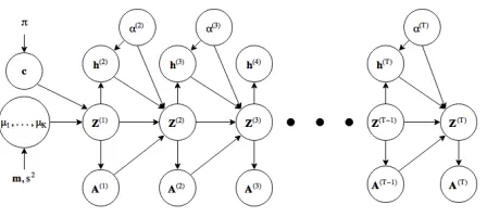
Figure 1: Graphical Model for ELSM.h(it) = 1for nodes that join the newly created community with centerα(t)and
0 otherwise. Thissplittingmechanism models the birth of new communities.
The parameter s1 dictates the spread within communities.
In the context of our example, this step corresponds to the creation of an initial set of political ideologies and individ-uals subscribing to these ideologies. Since µ1,µ2, ...,µK
are sampled independently, there will be at-mostKdistinct communities in latent space for the first time step. To encode prior information about communities in the model, rather than samplingµ1,µ2, ...,µK independently from a normal
distribution, one can specify these vectors explicitly.
2.2
Generating Observed
A
(t)from Latent
Z
(t)In ELSM, the probability of an edge between two nodes is inversely proportional to the distance between their dings in the latent space. By this, one hopes to get embed-dings that are easier to deal with for a clustering algorithm likek-means. We model this as follows:
a(ijt)=a(jit)∼Bernoullif(z(it)−z(jt)), i > j, (2)
where f(.) is a nonlinear function. The observed matri-ces are symmetric and we do not allow self loops. In our experiments on generation of synthetic networks, we used f(x) = 1−tanh(||x||2
2/s22), wheres2is a parameter that
controls the radius around a node’s embedding in the la-tent space within which it is more likely to connect to other nodes.
We will demonstrate via experiments in§5, that one can have other choices for the functionf(.)and the distribution parameterized by f(.)depending on problem context. For example, in the case of weighted graph with positive integer weights, Poisson distribution can be used.
2.3
Emergence of New Communities
If the nodes are only allowed to become similar to their neighbors, then over time the latent embeddings will col-lapse onto a single point and all the community structure in the network will be lost. But such a phenomenon is not ob-served in real world networks. In the absence of any other guiding force, to avoid the collapse of latent space and to model the emergence of new communities ELSM randomly generates a new community center at each time step.
At each time stept, a new community centerα(t)is
generate the original community centersµ1,µ2, ...,µK, i.e.
α(t)∼ N(m, s2I). We define a Bernoulli random variable h(it) for each node iat time t. If h(it) = 1, then node i’s updated latent embedding is sampled as:
z(it)∼ N(α(t), s21I) (3)
The parameters1has the same meaning as in (1). Ifh (t)
i =
0, then nodei’s latent embedding will be updated based on the embeddings of its neighbors at time stept−1 by the process described in the next subsection. We model the prob-abilityP(h(it) = 1)as a function of the distance between α(t)andz(t−1)
i . If the latent embedding of node iat time
stept−1 is close toα(t), thenP(h(t)
i = 1)will be high
and vice-versa. We model this as follows:
hi(t)∼Bernoullig(zi(t−1)−α(t)), (4)
where g(.) is a nonlinear function. In our experiments for generating synthetic data, we use g(x) = 1 −
tanh(||x||2
2/s23). The parameters3controls the influence of
the newly created community on other nodes. Note that this step does not necessarily involve the creation of a new com-munity as the sampledα(t)may lie within an existing com-munity in the latent space.
In the context of our example, this step will correspond to new political ideologies appearing in the latent space. Individuals that have a similar political ideology are more likely to embrace this new ideology. Individuals from differ-ent communities may come together and form a new politi-cal ideology of their own.
2.4
Evolving the Latent Space
ELSM tries to make nodes similar to their neighbors over time. To model this, for time stept = 2,3, ..., T, a mean vectorµ(it)is obtained for each nodeias follows:
µ(it)= 1 1 +P
j6=ia
(t−1)
ij l(z
(t−1)
i −z
(t−1)
j )
×z(it−1)
+X
j6=i
a(ijt−1)l(z(it−1)−z(jt−1))z(jt−1)
(5)
Here, we usel(x) =e−||x||2/s24 ands4 is a parameter that controls the influence of neighbors on a node. Note that only the immediate neighbors at timet−1can affect the future embedding of a node at timet. Also, note that the value of µ(it)lies in the convex hull formed by the embeddings of the node and its neighbors in the latent space a time stept−1. Ifh(it)= 0for a given node, then the updated embedding of the node is given by:
zi(t)∼ N(µi(t), s21I) (6)
Then, (3) and (6) can be combined to get the general update equation for the evolution of latent embeddings of the nodes as:
zi(t)∼ N(hi(t)α(t)+ (1−hi(t))µ(it), s21I), i= 1,2, ..., n (7)
Algorithm 1Generating Synthetic Networks Input:n,T,π,K,m,s,s1,s2,s3,s4
Sampleµ1,µ2, ...,µK∼ N(m, s2I)
Samplec1,c2, ...,cn∼π
SampleZ(1)using (1)
SampleA(1)using (2)
fort= 2toT do
Sampleα(t)∼ N(m, s2I)
Sampleh(t)using (4)
SampleZ(t)using (7)
SampleA(t)using (2)
end for
Return:{A(1),A(2), ...,A(T)}
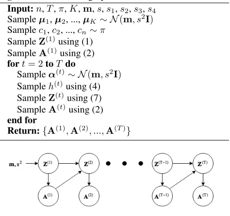
Figure 2: Graphical Model for iELSM
This not only allows the nodes to become similar over time, it also allows them to move apart to form new communities as it is observed in real world networks. In the context of our example, (5) says that an individual’s political ideology will be influenced by the political ideology of their peers.
It is easy to see that ELSM supports operations like birth, death, growth, shrinkage, merge and split on the commu-nities. The latent space offers a nice community structure (as we will show via our experiments, visualization of latent space is in supplementary material) because the operations presented in (2), (4) and (5) depend on distances between embeddings in the latent space. Figure 1 presents the under-lying graphical model for ELSM. The procedure for gener-ating synthetic networks is listed in Algorithm 1.
3
Inference Network
Inference is concerned with finding the latent embedding of each node at each time step,{Z(1),Z(2), ...,Z(T)}, that best
explains an observed dynamic network specified by the se-quence of adjacency matrices{A(1),A(2), ...,A(T)}. In this section, we describe the inference procedure for a simpli-fied version of ELSM. We argue that this simplisimpli-fied version, which we call Evolving Latent Space Model for Inference (iELSM), is as good as the original ELSM for the task of inference. Inference for ELSM follows along the same lines as iELSM and full details have been worked out in supple-mentary material.
3.1
Evolving Latent Space Model for Inference
apart over time and form new communities. In the absence of any other guiding force during the generation process, ELSM achieves this by the use of initial community cen-tersµ1,µ2, ...,µK, the initial membership vectorcand the
splitting mechanism as explained in§2.3.
However, during inference, given a sequence of observed adjacency matrices {A(1),A(2), ...,A(T)} for a dynamic network, the required guiding force is provided by the need to explain the observed data. In this case one need not in-corporate any of the elements mentioned above. Thus for the purpose of inference, we eliminate these elements and get a simplified model which we call iELSM. The graphical model for iELSM is shown in Figure 2. Note that iELSM also captures both the motivating phenomena (similar nodes connect more often and nodes become similar to their neigh-bors over time) mentioned in the beginning of§2.
The structures of probability distributions that govern iELSM are similar to the structures of corresponding dis-tributions in ELSM. The latent embeddingsz(it)follow (5) and (6) fori = 1,2, ..., nandt = 2,3, ..., T. The observed entriesa(ijt)follow (2). In addition we impose a prior on the first layer of latent embeddingsz(1)i fori= 1,2, ..., nas:
z(1)i ∼ N(m, s2I), (8)
Wheremandsare hyperparameters. We make the following independence assumptions:
1. The latent embeddings in the first layer z(1)i for i = 1,2, ..., nare independent.
2. a(ijt)is independent of everything else givenzi(t)andz(jt)
for alli, j= 1,2, ..., n, i6=jandt= 1,2, ..., T.
3. z(it)is independent of everything else given Z(t−1)and
A(t−1)fori= 1,2, ..., nandt= 2,3, ..., T
Since the observed adjacency matrices are assumed to be symmetric and self-loops are not allowed, we only need to consider the lower triangle (without the leading diagonal) in these matrices. The joint log likelihood for iELSM, which is given below, can then be computed using (2), (5), (6) and (8) as:
logP(A(1),Z(1),A(2),Z(2), ...,A(T),Z(T)) =
n
X
i=1
logP(z(1)i ) +
T
X
t=1
X
i>j
logP(a(ijt)|zi(t),z(jt))
+
T
X
t=2
n
X
i=1
logP(z(it)|Z(t−1),A(t−1))
(9)
3.2
Variational Inference for iELSM
Exact inference is intractable in iELSM because the ob-served entries ofA(t)do not follow a Gaussian distribution.
Thus, we resort to variational techniques (Blei, Kucukelbir, and McAuliffe 2017) to perform approximate inference. We use a LSTM based neural network to model the variational parameters. The neural network is then trained to maximize theELBOwhich we derive next.
We approximate the true posterior distribution P(Z(1),Z(2), ...,Z(T)|A(1),A(2), ...,A(T)) using a distribution Q(Z(1),Z(2), ...,Z(T);θ), where θ represents
parameters of a neural network. We further assume that Q(., θ) belongs to the mean-field variational family of distributions, i.e.:
Q(Z(1),Z(2), ...,Z(T);θ) =
T
Y
t=1
n
Y
i=1 qti(z
(t)
i ;θ) (10)
We model each factor qti(z
(t)
i ;θ) as a Gaussian
distribu-tion whose mean νi(t) ∈ Rd and variance (σ(t) i )2 ∈
Rd parameters are derived from the neural network. Here, as before, d is the dimension of latent space. Note that we have not explicitly shown the dependence of νi(t) and (σi(t))2 on θ to keep the notation clean. Let (σ(t)
i )
2I =
diag((σ(it))21,(σi(t))22, ...,(σi(t))2d), we can then write:
qti(z
(t)
i ;θ) =N(z
(t)
i |ν
(t)
i ,(σ
(t)
i )
2I) (11)
The objective is to maximize theELBOfunction which is given byEz∼q[logp(x,z)−logq(z)](Blei, Kucukelbir, and
McAuliffe 2017). Herexdenotes the observed variables,z
denotes the latent variables,p(x,z)is the joint distribution of x andz andq(z) is the distribution that approximates the posterior p(z|x). It can be shown thatELBOprovides a lower bound on the log probability of observed datap(x) (Kingma and Welling 2013), henceELBOcan be used as a surrogate function to maximize the probability of observed data. In our context,ELBOcan be written as:
ELBO(θ) =EZ(1),Z(2),...,Z(T)∼Q[
logP(A(1),Z(1), ...,A(T),Z(T))
−logQ(Z(1),Z(2), ...,Z(T);θ)]
(12)
The expectation of second term in (12) can be computed in closed form sinceQ(., θ)factorizes according to (10) and the factorsqti(.;θ)follow a Gaussian distribution. To
com-pute the expectation of first term, we use the Monte Carlo method to evaluate (9). In all our experiments, only one sam-ple was used to approximate the expectation of first term.
3.3
Network Architecture
Given the variational parameters νi(t) and (σ(it))2 for all i = 1,2, ..., nandt = 1,2, ..., T,ELBOcan be approx-imated using (12) as described above. In this section we describe the neural network architecture that parameterizes these quantities. There are two main advantages of this neu-ral network based approach: (i) neuneu-ral networks are pow-erful function approximates and hence complex node to la-tent embedding mappings can be learned and (ii) standard backpropagation algorithm with the reparameterization trick (Kingma and Welling 2013) can be used that allows efficient implementation.
Figure 3: Inference network architecture for iELSM.Mand
Vare neural networks that takegi(t)as input to produce the mean andlog-variance vectors respectively. Note that these networks are shared across all timesteps.
vector. The network updates its hidden state using the usual update rules for LSTM and produces an outputgi(t) ∈ Rm for each node. The outputg(it)is then used to produceνi(t) andlog (σi(t))2via the mean and variance networks (Mand
Vrespectively in Figure 3) that are shared across all time steps. Figure 3 shows the architecture of our inference net-work.
We use the reparameterization trick for Gaussian distribu-tion, as it was used in (Kingma and Welling 2013) to make the whole pipeline differentiable. This enables end to end training of the network. The embeddings sampled from this network can be used to compute (12) via Monte Carlo ap-proximation as it was discussed in§3.2. The objective is to maximizeELBO(θ)with respect to the parametersθof the inference network.
3.4
Encoder-Decoder View of the Inference
Network
The network given in Figure 3 can be seen as an encoder. At time stept, it takes the feature vector for each node (the row corresponding to that node in A(t)) as input and
pro-duces a time dependent embeddingz(it)for the node as out-put. Note that if observed node features are available, one can use these features in conjunction withA(t)as input to the network. A decoder should take these latent embeddings and try to reconstructA(t). By using (9) in (12), we obtain
a term that involveslogP(a(ijt)|zi(t),z(jt)). The estimator of this probability value acts as a simple decoder that tries to predict the probability of an observed edge given the latent embeddings of its two endpoints.
Recall from (2) that: (i) a(ijt) has been modeled by a Bernoulli distribution and (ii) The parameter for this Bernoulli distribution is given byf(z(it)−z(jt))where for generation we use f(x) = 1−tanh(||x||2
2/s22). One can
have a more complex decoder which utilizes problem spe-cific information. For example, the function f(x) can be modeled using a neural network. If the weights do not fol-low the Bernoulli distribution (i.e., the edges are weighted)
then one can use the problem context to enforce the right distribution on weights and learn the parameters of that dis-tribution accordingly. For example, in our experiments with Enron dataset, the edge weights are non-negative integers, so we model this by using a Poisson distribution and we use a neural network to learnf(x)so that it predicts the mean for the Poisson distribution.
This encoder-decoder view of the inference network makes the inference methodology very flexible. One can in-corporate domain knowledge to customize various compo-nents of this network so that it better suits the problem at hand.
4
Related Work
In general, dynamic networks, and in particular, link predic-tion and community detecpredic-tion in dynamic networks, have earned the attention of many researchers (Goldenberg et al. 2010; Kim et al. 2017). This can be attributed to the emer-gence of many practical applications (for e.g., social net-work analysis) where dynamic netnet-works are encountered.
An extension of Mixed Membership Stochastic Block Model (Airoldi et al. 2008) to the dynamic network setting by coupling it with a state-space model to capture temporal dynamics has been proposed in (Xing, Fu, and Song 2010; Ho, Song, and Xing 2011). Along the same lines, in (Yang et al. 2011), Stochastic Block Model (Holland, Laskey, and Leinhardt 1983) was extended by explicitly modeling transition between communities over time. Some other ap-proaches that extend a static network models are (Xu and Hero 2014; Xu 2015; Papadopoulos et al. 2012).
There have been many latent space based approaches for modeling dynamic networks. In (Sewell and Chen 2015; 2016) the transition of nodes’ latent embeddings is mod-eled independently for each node by using a Markov chain. In (Heaukulani and Ghahramani 2013), the authors intro-duced Latent Feature Propagation (LFP) that uses a dis-crete latent space and a HMM style latent embedding tran-sition model. In (Kim and Leskovec 2013) non-parametric Dynamic Multigroup Membership Graph model (DMMG) which additionally models the birth and death of communi-ties using Indian Buffet Process (Griffiths and Ghahramani 2011) has been introduced. The work of (Miller, Jordan, and Griffiths 2009; Foulds et al. 2011) are also along the same lines.
Most similar to our work, is the work done in (Heauku-lani and Ghahramani 2013; Kim and Leskovec 2013), how-ever there are significant differences as well. (i) While these approaches rely on MCMC, we use variational inference be-cause it offers many advantages as mentioned in (Blei, Ku-cukelbir, and McAuliffe 2017), (ii) We use a neural network to perform inference which allows an efficient implemen-tation and (iii) We have a more flexible, continuous latent space whereas these approaches use a discrete latent space.
5
Experiments
syn-thetic networks generated from ELSM and real world net-works. Our model outperforms existing methods on standard benchmarks. While we report the results for both ELSM and iELSM in§5.3 and§5.4, the inference procedure for ELSM has been described in supplementary material.
5.1
Synthetic Networks
We generated 10 synthetic networks using Algorithm 1. For each network, we used n = 100, T = 10,K = 5, π = [1/K, ...,1/K],m = [0,0]|,s = 1.0, s1 = 0.05, s2 = 0.2, s3 = 1.0 and s4 = 0.5 as input parameters.
Community detection was performed on these networks us-ing both normalized spectral clusterus-ing (von Luxburg 2007) and our inference network as described in§5.3. The scores reported in Table 1 for synthetic networks were obtained by averaging the scores across these 10 networks. Visualiza-tion of some generated networks and the corresponding la-tent spaces has been provided in supplementary material. A video that shows the evolution of latent space over time has also been attached as part of supplementary material.
5.2
Real World Networks
We evaluate our model on three real world dynamic net-works apart from evaluating it on synthetic netnet-works gen-erated by ELSM. This section describes the datasets that we have used for our experiments:
1) Enron email: The Enron dataset (Klimt and Yang 2004) contains emails that were exchanged between 149 in-dividuals over a period of three years. We use two different versions of this dataset - full and 50. Enron-full has 12 snapshots, one for each month of the year 2002. In snapshot t, entrya(ijt) counts the number of emails that were exchanged between usersi andj during that month. We also consider unweighted Enron-full obtained by making all snapshots binary. Following (Foulds et al. 2011), Enron-50 considers only top Enron-50 individuals with most number of emails across all snapshots. Each snapshot corresponds to a month (there are 37 snapshots). The adjacency matrix for each snapshot is symmetric and binary wherea(ijt) = 1if at least one email was exchanged between usersiandjduring that month and0otherwise.
2) NIPS co-authorship:There are 17 snapshots in this network, each corresponding to an year from 1987 to 2003. Entrya(ijt) counts the number of NIPS conference publica-tions in yeart, that have individualsiandj as co-authors. We use a subset of this dataset - NIPS-110, that is created by making the snapshots binary and selecting top 110 authors based on the number of unique co-authors that they have had over these 17 years (Heaukulani and Ghahramani 2013).
3) Infocom: This dataset contains information about physical proximity between 78 individuals over a 93 hours long interval at Infocom 2006. Following (Kim and Leskovec 2013), we create snapshots corresponding to 1 hour long intervals. At timet,a(ijt) = 1if both individuals iandjregistered each others physical proximity during the tthhour. We remove those snapshots that have fewer than 72
non-zero entries which leaves us with 50 snapshots.
We next describe the two tasks that we have performed on various subsets of these datasets, namely - community detection and link prediction.
5.3
Community Detection
The task is to assign each node to a community at each time step such thatsimilarnodes belong to the same community. To measure the quality of communities, at each time step, we use the well known modularity score. The modularity score lies in the range [−1/2,1), with values close to1 signify-ing goodcommunities (that have more edges within them as compared to the number of edges that will be obtained purely by chance).
We use the observed matrices {A(1),A(2), ...,A(T)}to
train the inference network for iELSM (§3.3) and ELSM (supplementary material). The latent embeddings obtained from the trained network are fed to the k-means clustering algorithm. At each time step, the optimal number of commu-nities,k(t)is chosen from the range[2,10]by selecting the
value ofk(t)that maximizes the modularity score on the
ad-jacency matrix that is induced by applying RBF kernel with variance parameter1to the latent space embeddings. Note that we do not use the original adjacency matrixA(t)while
selecting the optimal number of communities.
We experiment with different variants of decoder in the inference network. For Enron-full, the edges have positive integer weights, we model this by imposing a Poisson dis-tribution on P(a(ijt)|zi(t),z(jt)). Since iELSM (and ELSM) models the interaction between nodes as a function of dis-tance between their latent embeddings, we predict the mean of Poisson distribution for position(i, j)at time steptas:
ρij(t)= exp(−wρ2||zi(t)−z(jt)||2+b
ρ) (13)
The parameterswρ andbρ are shared across all time steps
and positions. These parameters are learned using standard backpropagation ((13) represents a single layer, single node neural network withexp(.)as the activation function). One can also employ a similar technique for learning parameters s2(§2.2) ands4(§2.4) from data by using a single layer,
sin-gle node neural network to learn optimal scaling of distances in (2) and (5).
The key claim that we wish to demonstrate here is that the latent embeddings learned by our model are not only good for finding communities at individual time steps, but also lead to a more plausible, gradually changing community structure over time. To do so, we compute the NMI score between community assignments at successive time steps. The NMI score lies in[0,1]with values close to1signifying gradual change in community structure in our setup.
We compare our scores against the scores obtained by independently applying normalized spectral clustering (von Luxburg 2007) at each snapshot. The number of communi-ties,k(t), is chosen by using the same method that was used for our model on the node embeddings produced by spectral clustering.
Table 1: Community Detection Results: It can be seen that the detected communities are meaningful (as evident by modularity scores that are comparable to the ones obtained by the spectral clustering algorithm) while at the same time beingsmooth(since the NMI scores are considerably higher) thereby validating our claim.
DATASET MODULARITY NMI
SPECTRAL iELSM (OURS) ELSM (OURS) SPECTRAL iELSM (OURS) ELSM (OURS)
SYNTHETIC .479 .489 .488 .769 .851 .864
ENRON
-FULL
(WEIGHTED)
.506 .597 .590 .455 .722 .823
ENRON
-FULL
(BINARY)
.540 .555 .551 .529 .767 .779
ENRON-50 .396 .419 .414 .560 .819 .838
NIPS-110 .497 .601 .595 .249 .804 .863
INFOCOM .283 .288 .270 .443 .643 .662
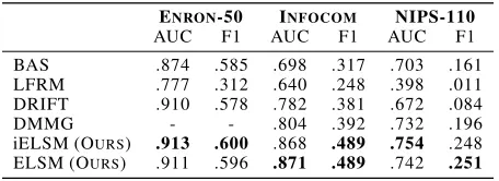
Table 2: Link Prediction Results: Our method outperforms other approaches on both metrics. We were unable to obtain an implementation for DMMG and hence the performance numbers of DMMG on Enron-50 are missing.
ENRON-50 INFOCOM NIPS-110
AUC F1 AUC F1 AUC F1
BAS .874 .585 .698 .317 .703 .161 LFRM .777 .312 .640 .248 .398 .011 DRIFT .910 .578 .782 .381 .672 .084
DMMG - - .804 .392 .732 .196
iELSM (OURS) .913 .600 .868 .489 .754 .248 ELSM (OURS) .911 .596 .871 .489 .742 .251
on the graph induced by latent embeddings, the scores re-ported in Table 1 correspond to the observed graph for the chosen number of communities. From Table 1, it is clear that our model achieves modularity scores that are at par (or better) with respect to spectral clustering while exhibiting a significantly higher NMI score, thus validating our claim.
5.4
Link Prediction
Good performance on community detection task testifies that the latent embeddings being learned by the network have a nice structure. But how does one ensure that the mod-eled network dynamics are faithful to real world data? Is our model overfitting to the training data to get good embed-dings? These questions get answered, if the observed data can be extrapolated to predict an unseen network snapshot using our model. This task is known as link prediction.
Formally, given network snapshots up to time t,
{A(1),A(2), ...,A(t)}, we want to predict the next network
snapshotA(t+1). Note that this involves predicting the
ap-pearance of new links as well as removal of existing links. We use binary networks in this experiment to compare against other approaches. We use the well known AUC score and F1 score for the purpose of comparison. Values close to 1indicate good performance for both the scores.
To predict A(t+1), we train the inference network for
iELSM and ELSM on{A(1),A(2), ...,A(t)}. We update the
predicted latent embeddings Z(t) using (5) and (6) to get
Z(t+1). Then, P(aij(t+1) = 1|Z(t+1)) is computed using
(2) (or the decoder, if a decoder network has been used). Note that for ELSM, while updating the latent embeddings we seth(it+1)= 0for all nodes.
We compare our performance against a simple baseline (BAS) in which the probability of an edge is directly pro-portional to the number of times it has been observed in the past (Foulds et al. 2011). We also compare against existing approaches - LFRM (Miller, Jordan, and Griffiths 2009) (us-ing only the last snapshot), DRIFT (Foulds et al. 2011) and DMMG (Kim and Leskovec 2013) (Table 2). Maximum F1 score over all thresholds is selected at each snapshot as it was done in (Kim and Leskovec 2013). The scores reported here have been obtained by averaging the snapshot wise scores. It can be seen that our method outperforms other methods on both metrics. Visualization of latent embeddings and pre-dicted output matrices for Enron-full can be found in sup-plementary material.
6
Conclusion and Future Work
In this paper, we proposed ELSM, a generative model for dynamically evolving networks. We also proposed a neu-ral network architecture that performs approximate infer-ence in a simplified version of our model, iELSM (inferinfer-ence for ELSM is in supplementary material) and highlighted the flexibility of this approach. Our model is capable of: (i) Gen-erating synthetic dynamic networks with gradually evolv-ing communities and (ii) Learnevolv-ing meanevolv-ingful latent embed-dings of nodes in a dynamic network. We demonstrated the quality of learned latent embeddings on downstream tasks like community detection and link prediction in dynamic networks.
a large number of real world networks, there are other im-portant classes of networks that do not follow these proper-ties. For example, one can also extend this idea to directed networks. One can also consider the case where the number of nodes is allowed to change over time. Considering net-works that are not necessarily assortative (like hierarchical networks) also poses interesting questions.
References
Airoldi, E. M.; Blei, D. M.; Fienberg, S. E.; and Xing, E. P. 2008. Mixed membership stochastic blockmodels. Journal of Machine Learning Research (JMLR)9:1981–2014. Blei, D. M.; Kucukelbir, A.; and McAuliffe, J. D. 2017. Variational inference: A review for statisticians. Journal of the American Statistical Association112(518):859–877. Fortunato, S. 2010. Community detection in graphs.Physics Reports486(3):75 – 174.
Foulds, J.; DuBois, C.; Asuncion, A.; Butts, C.; and Smyth, P. 2011. A dynamic relational infinite feature model for lon-gitudinal social networks.Proceedings of Machine Learning Research (PMLR)15:287–295.
Goldenberg, A.; Zheng, A. X.; Fienberg, S. E.; and Airoldi, E. M. 2010. A survey of statistical network models. Foun-dations and Trendsrin Machine Learning2(2):129–233. Griffiths, T. L., and Ghahramani, Z. 2011. The indian buffet process: An introduction and review. Journal of Machine Learning Research (JMLR)12:1185–1224.
Gupta, S.; Sharma, G.; and Dukkipati, A. 2018. A generative model for dynamic networks with applications: Supplemen-tary material.ArXiv e-prints1802.03725.
Heaukulani, C., and Ghahramani, Z. 2013. Dynamic prob-abilistic models for latent feature propagation in social net-works. InProceedings of the 30th International Conference on Machine Learning (ICML).
Ho, Q.; Song, L.; and Xing, E. P. 2011. Evolving cluster mixed-membership blockmodel for time-varying networks. Journal of Machine Learning Research (JMLR) 15:342– 350.
Holland, P. W.; Laskey, K. B.; and Leinhardt, S. 1983. Stochastic blockmodels: First steps. Social Networks 5(2):109 – 137.
Kim, M., and Leskovec, J. 2013. Nonparametric multi-group membership model for dynamic networks. Advances in Neural Information Processing Systems26:1385–1393. Kim, B.; Lee, K.; Xue, L.; and Niu, X. 2017. A review of dynamic network models with latent variables. CoRR. Kingma, D. P., and Welling, M. 2013. Auto-encoding vari-ational bayes. Proceedings of the 2nd International Confer-ence on Learning Representations (ICLR).
Klimt, B., and Yang, Y. 2004. The enron corpus: A new dataset for email classification research. InIn Proceedings of the European Conference on Machine Learning (ECML), volume 3201.
Miller, K.; Jordan, M. I.; and Griffiths, T. L. 2009. Nonpara-metric latent feature models for link prediction.Advances in Neural Information Processing Systems22:1276–1284.
Papadopoulos, F.; Kitsak, M.; Serrano, M. n.; Bogu˜n´a, M.; and Krioukov, D. 2012. Popularity versus similarity in growing networks.Nature489.
Rossetti, G., and Cazabet, R. 2017. Community discovery in dynamic networks: A survey.CoRRabs/1707.03186. Sewell, D. K., and Chen, Y. 2015. Latent space models for dynamic networks. Journal of the American Statistical Association110(512):1646–1657.
Sewell, D. K., and Chen, Y. 2016. Latent space models for dynamic networks with weighted edges. Social Networks 44:105 – 116.
von Luxburg, U. 2007. A tutorial on spectral clustering. Statistics and Computing17(4):395–416.
Xing, E. P.; Fu, W.; and Song, L. 2010. A state-space mixed membership blockmodel for dynamic network tomography. The Annals of Applied Statistics4(2):535–566.
Xu, K. S., and Hero, A. O. 2014. Dynamic stochastic block-models for time-evolving social networks. IEEE Journal of Selected Topics in Signal Processing8(4):552–562. Xu, K. S. 2015. Stochastic block transition models for dy-namic networks. Journal of Machine Learning Research (JMLR)38:1079–1087.