Long-term trends in the relation between daytime and nighttime values of fo F2

Ann. Geophys., 26, 1199–1206, 2008 www.ann-geophys.net/26/1199/2008/ © European Geosciences Union 2008

Annales

Geophysicae

Long-term trends in the relation between daytime and nighttime

values of foF2

A. D. Danilov

Institute of Applied Geophysics, Rostokinskaya 9, Moscow, 129128, Russia

Received: 10 May 2007 – Revised: 3 January 2008 – Accepted: 3 January 2008 – Published: 28 May 2008

Abstract. The data from the vertical ionospheric sounding for 12 stations over the world were analyzed to find the rela-tion between the values of foF2 for 02:00 LT and 14:00 LT of the same day. It is found that, in general, there exists a negative correlation between foF2(02) and foF2(14). The value of the correlation coefficientR(foF2) can be in some cases high enough and reach minus 0.7–0.8. The value of R(foF2) demonstrates a well pronounced seasonal variations, the highest negative values being observed at the equinox pe-riods of the year. It is also found thatR(foF2) depends on geomagnetic activity: the magnitude ofR(foF2) is the high-est for the choice of only magnetically quiet days (Ap<6),

decreasing with the increase of the limiting value of Ap.

For a fixed limitation onAp, the value ofR(foF2) depends

also on solar activity. Apparently, the effects found are re-lated to thermospheric winds. Analysis of long series of the vertical sounding data shows that there is a long-term trend inR(foF2) with a statistically significant increase in the R(foF2) magnitude after about 1980. Similar analysis is per-formed for the foF2(02)/foF2(14) ratio itself. The ratio also demonstrates a systematic trend after 1980. Both trends are interpreted in terms of long-term changes in thermospheric circulation.

Keywords. Ionosphere (Ionosphere-atmosphere interac-tions; Mid-latitude ionosphere)

1 Introduction

The problem of long-term changes (trends) in the ionosphere is an object of a close attention of specialists in various sci-entific groups (see the summarizing paper by Lastovicka et al., 2006). In spite of many efforts applied, there is still no common opinion either on the values of the trends in F2-Correspondence to: A. D. Danilov

([email protected])

region parameters, or on their origin (for details see Las-tovicka et al., 2006). Various mechanisms are considered including greenhouse gases increase, long-term changes in geomagnetic activity, and anthropogenic changes in the ther-mosphere. All of these mechanisms may impact the F2-layer parameters via both, changes in photochemical (composi-tion, temperature) or dynamical (circula(composi-tion, vertical drift) parameters of the thermosphere.

Till now all the studies of trends in the F2 region were aimed at the analysis of long-term behavior either of foF2 or hmF2. The main goal of this paper is to try to take a look at the trends in the relation between the nighttime and daytime values of foF2. The reason for such an attempt is that foF2 in the daytime and at night is governed by different processes: photochemistry and composition changes dom-inate in the daytime, whereas dynamical processes (vertical drift induced mainly by the horizontal circulation) govern the nighttime values of foF2.

Vanina-Dart and Danilov (2006) were the first to draw at-tention to the fact that there is a significant negative corre-lation between the nighttime and daytime values of foF2 for the same day. Danilov (2006) described the phenomenon in detail. It was found that the correlation coefficientR(foF2) between the nighttime and daytime values of foF2 for the same day is negative and can by the magnitude reach val-ues of 0.8–0.9. Analyzing the data of a dozen of ionospheric stations, Danilov (2006) studied the main features of the ef-fect. The detailed description of all the features of the phe-nomenon is out of the scope of this paper and we refer the reader to the above paper. Here we briefly describe only the main points important for the problem of deriving long-term trends inR(foF2).

1200 A. D. Danilov: Long-term trends in the relation between daytime and nighttime values of foF2

Table 1. List of ionospheric stations mentioned in the paper.

Station Coordinates Station Coordinates Geogr. Geom. Geogr. Geom.

Dourbes 50 N 5 E 52 N Leningrad 60 N 31 E 56 N Hobart 43 S 147 E 51 S Moscow 56 N 37 E 51 N Juliusruh 55 N 14 E 54 N Poitiers 47 N 0 E 49 N Gorky 56 N 44 E 59 N Slough 52 N 0 E 54 N Kaliningrad 55 N 21 E 53 N Tomsk 57 N 85 E 46 N

0 2 4 6 8 10 12 Months

-0.8 -0.4 0.0 0.4

R(

fo

F

2

)

1980 Kaliningrad

Ap<8

99%

Slough Tomsk

0

Fig. 1. Variations inR(foF2) over the year for 3 stations: Kalin-ingrad (circles), Slough(diamonds), and Tomsk (triangles). Hori-zontal dashed lines show the values ofR(foF2) needed to provide a 99% confidence level according to the Fisher’s F parameter test.

the point for April in Fig. 1 corresponds to the correlation between the nighttime and daytime values of foF2 calculated for the March–May period. The calculations were performed for different levels of magnetic activity (Ap<6, 12, 16, 20,

30, and 40). In each case only the days withAplower than

the particular value were taken for the calculation ofR(foF2). The list of stations mentioned in this paper is presented in Ta-ble 1.

Figure 1 shows the seasonal behavior ofR(foF2) for three stations forAp<8. First, one can see a strong similarity in

theR(foF2) behavior with time for all three stations. This fact increases the reliability of the effect, because three abso-lutely independent sets of data provide the same picture.

The main feature of Fig. 1 is the presence of two pro-nounced maxima in the magnitude ofR(foF2) in spring and fall. The absolute value ofR(foF2) in spring for Tomsk and Kaliningrad stations reaches about 0.6 and exceeds the value providing the 99% significance by the Fisher F parameter test (Pollard, 1977). The fall maximum in theR(foF2) magnitude is lower,R(foF2) being about−02 to−03. Principally the same picture was obtained for all stations and all limitations overApconsidered. In some cases the fall maximum was of

the same magnitude (or even slightly higher) then the spring

10 20 30

Upper limit of Ap

0.30 0.40 0.50 0.60 0.70 0.80

-R

(f

o

F

2

)

Kaliningrad

Moscow 1980

R =0.94

R = 0.87

0 2

2

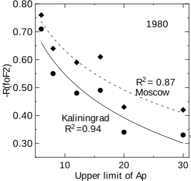
Fig. 2. Variations ofR(foF2) with the limiting value of theApindex

for two stations.

one, but in the majority of cases the spring maximum dom-inated. Some sort of a maximum (but with positive values ofR(foF2)) is seen in Fig. 1 at the solstices. However, the summer maximum is low and of low statistical significance. As for the winter maximum, the magnitude ofR(foF2) can in some cases reach 0.4–0.5, but never be as high as that for the equinox maxima (0.7–0.8). No special analysis has been performed for the solstice maxima.

2 Trends in theR(foF2) value

To characterize each year for the particular station and lim-itation in magnetic activity we took the maximum negative value ofR(foF2) regardless the season it was obtained. For the sake of comparison we considered also taking only the spring (March–April) values and found that principally the results are the same, but the statistics is certainly better in the former case.

The dependence ofR(foF2) for two stations on geomag-netic activity (on the limiting value ofAp,Ap(lim)) for 1980

is shown in Fig. 2. The magnitude of R(foF2) is seen to increase with the decrease in Ap(lim). In other words, the

quieter the days we choose, the better is pronounced the neg-ative correlation between foF2(02) and foF2(14). If only very quiet days (Ap<6) are chosen for the calculation ofR(foF2),

the magnitude of the latter exceeds 0.7, whereas atAp<30

it is 0.35–0.40. The approximation by a logarithmic function is shown by lines in Fig. 2. TheR2values show the determi-nation coefficients for the approximation lines.

Figures similar to Figs. 1 and 2 were calculated for all the stations and thresholds inAp considered. The principal

A. D. Danilov: Long-term trends in the relation between daytime and nighttime values of foF2 1201 To look for possible long-term trends inR(foF2) we had to

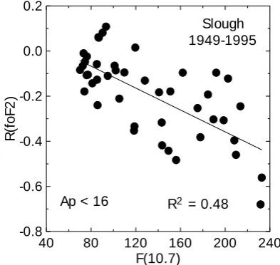
remove theR(foF2) dependence on solar activity. Such de-pendence exists (see Fig. 3 for Slough) though with the scat-ter of points, part of which may be due to the trends we are looking for. To remove the solar activity effects, we applied a simple method used in many publications on trends in the F2 region (see Bremer, 1998). We drew a regression line (solid line in Fig. 3) and for each point took the deviation from it:1R(foF2)=R(foF2)(obs)–R(foF2)(reg),R(foF2)(obs) and R(foF2)(reg) being the values of R(foF2) obtained by the method described above and corresponding to the regression line, respectively.

The time behavior of1R(foF2) for Hobart and Dourbes stations is shown in Fig. 4. One can see that there is a scatter of the1R(foF2) values before 1979 with poorly pronounced variation with time. After 1979 the picture looks different: there is a pronounced (R2=0.52 and 0.41) decrease in the 1R(foF2) value with time. The decrease is statistically sig-nificant at the 99% confidence level according to the Fisher F parameter test. The decrease in1R(foF2) means an increase in the magnitude ofR(foF2).

Similar pictures were obtained for other stations analyzed. Examples of 1R(foF2) variations with time for Juliusruh and Slough are presented in Fig. 5 and for Kaliningrad and Moscow in Fig. 6. One can see that the determination coef-ficientR2after about 1980 is high enough and provides the confidence level of 99% according to the Fisher F parameter test.

The boundary between the two regions with different 1R(foF2) behavior only slightly differs for all the stations considered and corresponds to 1978–1982. Thus, we see a systematic change at all stations: after about 1980 the neg-ative correlation coefficient between the daytime and night-time values of foF2 increase by the magnitude.

Some indications of the existence of periods of growth and decline inR(foF2) may be found also before 1980. Figure 7 shows the 132-month smoothed values of theAp index

ac-cording to Mikhailov et al. (2002) (top panel) and values of 1R(foF2) for Slough station smoothed in the same way (see also Fig. 4). One can see that the behavior of1R(foF2) re-peats the behavior of Ap(smooth) with a delay of about 3

years. That is exactly what Mikhailov et al. (2002) found for the behavior of hmF2 at Slough station.

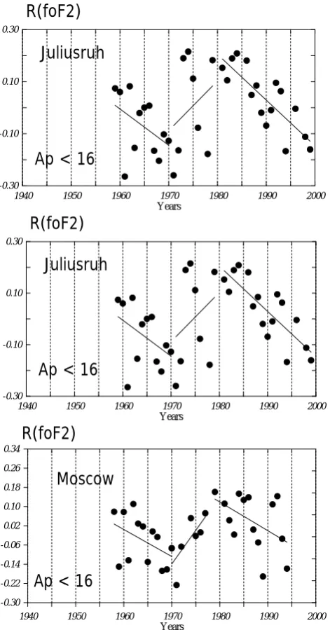
Figure 8 shows the behavior of 1R(foF2) for Gorky, Juliusruh, and Moscow stations. No smoothing has been ap-plied. Just the points were approximated by a linear regres-sion for 1970–1980 and for years before 1970. The only aim of this action is to show that there is a similarity in the time behavior of1R(foF2) for these three stations with the time behavior of the smoothed values ofAp. Comparing Fig. 8

with the top panel of Fig. 7, one can see that even without the 132-month smoothing (as in the case of Slough) the time behavior of 1R(foF2) with considerable scatter shows the same features as the time behavior ofAp(smooth). The

lat-ter fact suggests that the long-lat-term variations inR(foF2) (at

40 80 120 160 200 240 F(10.7)

-0.8 -0.6 -0.4 -0.2 0.0 0.2

R(

fo

F

2

)

Slough

R = 0.482

1949-1995

Ap < 16

Fig. 3. TheR(foF2) dependence on the solar activity index F(10.7) for Slough.

least, before 1980) may be caused by the long-term varia-tions in magnetic activity as was suggested by Mikhailov et al. (2002) for foF2 variations.

3 Trends in the foF2(02)/foF2(14) value

The second step of the analysis was to consider the behav-ior of the ratio of the critical frequencies foF2(02)/foF2(14) itself.

The annual variations in foF2(02)/foF2(14) presented nothing unexpected with a slight maximum in the ratio in June–July. So the average of the foF2(02)/foF2(14) values for these two months and for January-February was taken for each year in further searches for long-term trends.

As to the dependence on geomagnetic activity, it appeared to be quite different from that forR(foF2). Figure 9 shows variations with Ap(lim) of R(foF2) and foF2(02)/foF2(14)

for Slough for the fall period. One can see that the behavior ofR(foF2) is the same as shown in Fig. 2 for Kaliningrad and Moscow (the magnitude ofR(foF2) increases with a decrease ofAp(lim)), whereas foF2(02)/foF2(14) shows no significant

dependence onAp(lim).

The different behavior ofR(foF2) and foF2(02)/foF2(14) shown in Fig. 9 is easily understood in the scope of the con-cept considered. Variations in intensity and even direction of the meridional wind (which are especially frequent around equinoxes) would change the foF2(02)/foF2(14) ratio in both directions, but the average value for the days with the cho-senAp(lim) over three months would not vary considerably.

1202 A. D. Danilov: Long-term trends in the relation between daytime and nighttime values of foF2

1950 1960 1970 1980 1990 2000

years

-0.4 0.0

0.4 1950-1999

Hobart

Ap < 16 R =0.52

R(foF2) Δ

2

1960 1970 1980 1990 2000

years -0.4

0.0 0.4

Dourbes 1958-1997 Ap < 16

R =0.41 R(foF2)

Δ

2

Fig. 4. Variations with time of the1R(foF2) for Hobart and Dourbes.

1960 1970 1980 1990 2000

years

-0.4 0.0

0.4 1958-1999 Juliusruh

Ap < 16 R =0.42 R(foF2)

Δ

2

1950 1960 1970 1980 1990

years -0.4

-0.2 0.0 0.2 0.4

Slough 1949-1995

Ap < 16

R =0.36 R(foF2)

Δ

2

0

Fig. 5. Variations with time of the1R(foF2) for Juliusruh and Slough.

In the same way asR(foF2), the foF2(02)/foF2(14) value depends on solar activity. Figure 10 shows this dependence for Moscow forAp<30. One can see that the dependence

of foF2(02)/foF2(14) on solar activity index F(10.7) is much better pronounced and statistically significant than that for R(foF2) (see above Fig. 3).

In the same way as it has been done above forR(foF2), to get rid of the dependence on solar activity, the1fo(02)/fo(14) value has been found as the deviation of each particular point in Fig. 10 from the approximation line.

A detailed analysis of the 1foF2(02)/foF2(14) behavior was presented by Danilov (2008)1. A detailed description of the results is outside the frame of this paper. We note only that analyzing the data of 42 ionospheric stations, it was found that principally the situation is similar to that with1R(foF2) (see Figs. 4–6): after about 1980 the value of 1fo(02)/fo(14) demonstrate a systematic variation with 1_{Danilov, A. D.: Time and spatial variations of the}

A. D. Danilov: Long-term trends in the relation between daytime and nighttime values of foF2 1203

1970 1980 1990

years -0.4

-0.2 0.0 0.2 0.4

Kaliningrad 1965-1994

Ap < 16

R =0.472

R(foF2)

Δ

0

1960 1970 1980 1990

years -0.2

0.0 0.2

Moscow 1958-1994

Ap < 16 R =0.53

0

2

R(foF2) Δ

Fig. 6. Variations with time of1R(foF2) for Kaliningrad and Moscow (Ap<16).

time (a decrease or increase) which is statistically signifi-cant at the 95–99% confidence level according to the Fisher’s F parameter test. Figures 11, 12, and 13 show examples of the time behavior of the 1foF2(02)/foF2(14) value for some stations. Danilov (2008)1 found also that the sign of the1foF2(02)/foF2(14) changes after about 1980 is related to the magnetic inclination and declination of the station. That made it possible to postulate that the observed effect is caused by systematic changes in the zonal wind in the ther-mosphere (Danilov, 20081).

The analysis shows that, unlike in Figs. 7 and 8, no system-atic behavior resembling theAp132 long-term behavior can

be found in the 1foF2(02)/foF2(14) behavior before about 1980.

This difference in the behavior of R(foF2) and foF2(02)/foF2(14) with time before 1980 is understandable if one takes into account the result illustrated by Fig. 9 above. The latter shows that R(foF2) is very sensitive to changes in geomagnetic activity, whereas foF2(02)/foF2(14) is not. Respectively, there is a pronounced signature of magnetic activity long-term variations inR(foF2) behavior during the decades preceding 1980, whereas there is no such signature in the foF2(02)/foF2(14) behavior.

The trend in the correlation coefficientR(foF2) after about 1980, considered above in this paper, presumably indicate systematic changes in the meridional wind in the thermo-sphere. The 1foF2(02)/foF2(14) behavior after 1980 was shown by Danilov (2008)1to indicate to systematic change in the zonal wind. So one can assume that there is a change in the dynamical regime of the thermosphere. At the moment, one cannot say what causes this change. The latter may be

1940 1950 1960 1970 1980 1990 2000 10

12 14 16 18 20

Ap

11-year running mean Ap

1940 1950 1960 1970 1980 1990 2000

Years

-0.22 -0.14 -0.06 0.02 0.10 0.18 0.26 0.34

Slough

Ap < 16

R(foF2)

Δ

Fig. 7. Comparison of the 132-month smoothed values ofApand

1R(foF2) for Slough.

1204 A. D. Danilov: Long-term trends in the relation between daytime and nighttime values of foF2

1940 1950 1960 1970 1980 1990 2000

Years

-0.30 -0.10 0.10 0.30

Juliusruh

Ap < 16

R(foF2)

Δ

1940 1950 1960 1970 1980 1990 2000

Years

-0.30 -0.10 0.10 0.30

Juliusruh

Ap < 16

R(foF2)

Δ

1940 1950 1960 1970 1980 1990 2000

Years

-0.30 -0.22 -0.14 -0.06 0.02 0.10 0.18 0.26 0.34

Moscow

R(foF2)

Δ

Ap < 16

Fig. 8. Time behavior of 1R(foF2) for Gorky, Juliusruh, and Moscow.

gas amount. In the majority of papers, the impact of this in-crease on the middle and upper atmosphere is considered via the changes in neutral temperature. However, it seems to be inevitable that such changes (different at different heights) should lead to changes in the global circulation pattern, in-cluding the meridional and zonal winds at thermospheric heights.

10 20 30

Ap Upper Limit 0.4

0.5 0.6

--R

(fo

F

2

);

fo

(0

2)

/

fo

(14

)

1970 Slough

ratio R

October

0

Fig. 9. Variations with the limiting value ofAp inR(foF2) and

foF2(02)/foF2(14) for the fall period of 1970 at Slough.

40 80 120 160 200 240

F(10.7)

0.60 0.64 0.68 0.72 0.76 0.80

fo

(0

2)

/

fo

(14)

Moscow Ap <30

R =0.87 June/ July

1958-1979

2

Fig. 10. The fo(02)/fo(14) dependence on the solar activity index

F(10.7) for Moscow. Solid line shows the approximation of the points by a 3rd degree polynomial.

4 Conclusions

The analysis of long-term trends in the relation between the daytime and nighttime values of foF2 is performed in two ways. Consideration of the correlation coefficient R(foF2) between foF2(02) and foF2(14) (the values of foF2 for 02:00 LT and 14:00 LT) shows thatR(foF2) is negative in spring and fall and has a maximum in magnitude (most often in spring) reaching 0.8–0.85. The coefficient is very sensitive to magnetic activity: with theAp threshold of the

A. D. Danilov: Long-term trends in the relation between daytime and nighttime values of foF2 1205

1960 1970 1980 1990

Years

-0.04 -0.02 0.00 0.02 0.04

Moscow

R =0.67

June/July

fo(02)/ fo(14)

Δ

2

0

1960 1970 1980 1990 2000 years

-0.08 -0.04 0.00 0.04 0.08

Slough

R =0.42 1958-1995

Jan/ Feb

fo(02)/ fo(14)

2

Fig. 11. Time behavior of1foF2(02)/foF2(14) for Moscow and Slough.

1960 1970 1980 1990 2000 Years

-0.04 0.00 0.04

Poitiers

R =0.60 June/ July 1958-1997

2

fo(02)/ fo(14)

Δ

1950 1960 1970 1980 1990 2000

Years

-0.04 -0.02 0.00 0.02

0.04 _1958-1998Dourbes

R = 0.812

fo(02)/ fo(14) Δ

June/ July

Fig. 12. Time behavior of1foF2(02)/foF2(14) for Poitiers and Dourbes.

ofR(foF2) demonstrates the same feature: after about 1980 the magnitude of negativeR(foF2) increases.

Looking for an explanation of the existence of the nega-tive correlation coefficient and the features of its behavior de-scribed above, we offer the following proposal. The daytime value of NmF2 (i.e. foF2) increases with an intensification of the poleward meridional wind because the latter increases values of the atomic oxygen concentration. The same wind shifts the F2-layer maximum along the magnetic field lines down to lower altitudes into the region of higher recombi-nation and so leads to a decrease in the nighttime values of NmF2. The equatorward meridional circulation leads to the

opposite effect for both, the daytime and nighttime values of NmF2. Thus, changes in the meridional wind should lead to opposite changes in the daytime and nighttime values of foF2, providing negative correlation between these values.

1206 A. D. Danilov: Long-term trends in the relation between daytime and nighttime values of foF2

1960 1970 1980 1990 2000 years

-0.08 -0.04 0.00 0.04

Leningrad

R =0.53 1958-1998

June/ July

2

fo(02)/ fo(14) Δ

1950 1960 1970 1980 1990 2000 years

-0.08 -0.04 0.00 0.04

Tomsk

R =0.54 1958-1997

June/ July fo(02)/ fo(14)

Δ

2

Fig. 13. Time behavior of1fo(02)/fo(14) for Leningrad and Tomsk.

The dependence of R(foF2) on the magnetic activity threshold (see Fig. 2) is also understandable. The effect of the changes in the meridional wind intensity and direction should be the more pronounced the quieter the geomagnetic situation. In geomagnetically disturbed conditions, the sim-ple scheme described is distorted by the influence of the heat-ing in the auroral oval, which counteracts poleward wind, leading to changes not only in the meridional circulation, but in the composition and temperature of the thermospheric gas at F2-region heights, as well.

In the scope of the concept described, the systematic in-crease of the magnitude ofR(foF2) after about 1980 suggests that since this date there was a systematic intensification of the meridional circulation.

The behavior ofR(foF2) before 1980 demonstrates some similarity with the behavior of the smoothed values ofAp

used by Mikhailov et al. (2002) to derive trends in foF2. This similarity leads to the conclusion that the changes in the cir-culation may be due to the long-term magnetic activity ef-fects.

The same analysis was performed for the foF2(02)/foF2(14) ratio itself. The ratio demonstrates no pronounced dependence on the choice of magnetically quiet days. After about 1980 a systematic change in the foF2(02)/foF2(14) value is found for all stations considered (Danilov, 20081). These changes are presumably related to changes in the zonal thermospheric wind. Jointly, the analysis of the data on R(foF2) and foF2(02)/foF2(14) indicate changes in the thermospheric circulation at F-region heights after about 1980. The cause of these changes is not clear yet. It may be an indirect effect of the long-term changes in magnetic activity, or a manifestation of long-term changes in the dynamical regime of the upper atmosphere resulting from anthropogenic impact.

Acknowledgements. The author thanks A. V. Mikhailov for creation of computer programs required and for a fruitful discussion of the results and a Reviewer, P. Wilkinson for vary valuable comments and corrections of the language. The work was supported by the Russian Foundation for Basic Research (project No. 04-05-64832). Topical Editor M. Pinnock thanks P. Wilkinson and another anonymous referee for their help in evaluating this paper.

References

Bremer, J.: Trends in the ionospheric E and F regions over Europe, Ann. Geophys., 16, 986–996, 1998,

http://www.ann-geophys.net/16/986/1998/.

Danilov, A. D.: Relation between daytime and night-time values of the critical frequency foF2, Int. J. Geomagn. Aeron., 6(3), GI3003, doi:10.1029/2005GI000129, 2006.

Laˇstoviˇcka, J., Ulich, T., Bremer, J., Elias, A. G., Ortiz de Adler, N., Jara, V., Abarca del Rio, R., Floppiano, A. J., Ovalle, E., and Danilov, A. D.: Long-term trends in foF2: a comparison of various methods, J. Atmos. Solar-Terr. Phys., 68, 1854–1870, 2006.

Mikhailov, A. V., Marin, D., Leshchinskaya, T. Yu., and Herraiz, M.: A revised approach to the foF2 long-term trends analysis, Ann. Geophys., 20, 1663–1675, 2002,

http://www.ann-geophys.net/20/1663/2002/.

Pollard, J. H.: A Handbook of Numerical and Statistical Tech-niques, Cambridge University Press, Cambridge, 1977. Vanina-Dart, L. B. and Danilov, A. D.: Relation between the