The wave surveyor technique for fast plasma wave detection in multi-spacecraft data

www.ann-geophys.net/26/1699/2008/ © European Geosciences Union 2008

Annales

Geophysicae

The wave surveyor technique for fast plasma wave detection in

multi-spacecraft data

J. Vogt1, Y. Narita2, and O. D. Constantinescu2

1_{School of Engineering and Science, Jacobs University Bremen, Campus Ring 1, 28759 Bremen, Germany}

2_{Institut f¨ur Geophysik und extraterrestrische Physik, Technische Universit¨at Braunschweig, Mendelssohnstr. 3, 38106} Braunschweig, Germany

Received: 19 November 2007 – Revised: 17 March 2008 – Accepted: 18 April 2008 – Published: 18 June 2008

Abstract. Multi-satellite missions like Cluster allow to study the full spatio-temporal variability of plasma processes in near-Earth space, and both the frequency and the wave vector dependence of dispersion relations can be reconstructed. Ex-isting wave analysis methods include high-resolution beam-formers like the wave telescope ork-filtering technique, and the phase differencing approach that combines the correla-tions measured at pairs of sensors of the spacecraft array. In this paper, we make use of the eigendecomposition of the cross spectral density matrix to construct a direct wave iden-tification method that we choose to call the wave surveyor technique. The analysis scheme extracts only the dominant wave mode but is much faster to apply than existing tech-niques, hence it is expected to ease survey-type detection of waves in large data sets. The wave surveyor technique is demonstrated by means of synthetic data, and is also applied to Cluster magnetometer measurements.

Keywords. Space plasma physics (Turbulence; Waves and instabilities; Instruments and techniques)

1 Introduction

Near-Earth space is a dynamic plasma environment that cre-ates and supports wave activity on a broad range of tem-poral and spatial scales. The inherent ambiguity of single-spacecraft data makes it difficult to identify waves as, e.g. Doppler shifts may significantly affect the frequency deter-mination. Multi-satellite missions can overcome this prob-lem.

Estimation of wave vectorskfrom such multipoint mea-surements, however, is not as straightforward as a Fourier transformation because of the small number of sensors in the Correspondence to: J. Vogt

([email protected])

spacecraft array. In the context of the Cluster mission, sev-eral approaches to the problem have been presented. Dunlop et al. (1988) and Neubauer and Glassmeier (1990) introduced the term wave telescope for a method based on a linear filter bank approach, and quantified the spatial aliasing condition in terms of the reciprocal lattice of the spacecraft tetrahe-dron. Thek-filtering technique constructed by Pincon and co-workers (e.g. Pincon and Lefeuvre, 1991, 1992; Pincon and Motschmann, 1998) by means of a minimization prin-ciple is based on an estimator for the spatio-temporal power spectrumP (ω,k). Sensor weights are chosen such that the contribution of plane waves with wave vectorsk0 _{outside a}

small spectral window aroundkto the resulting spectral en-ergy density estimator is minimum. Such techniques were originally developed for seismic arrays (e.g. Capon et al., 1967; Capon, 1969; Cox, 1973), and are commonly referred to as Capon estimators, minimum variance estimators, high resolution beamformers or simply beamformers. Minimum variance estimators have been used to identify MHD waves in the magnetosheath and the foreshock region (Glassmeier et al., 2001; Narita et al., 2003; Narita and Glassmeier, 2005) and to study turbulence (Sahraoui et al., 2003, 2006; Narita et al., 2006). Furthermore, Constantinescu et al. (2007) con-structed a wave detection scheme based on spherical waves instead of plane waves to identify not only wave vectors but also the location of the wave source.

the observed signals. In the preparation phase of the Cluster mission, the phase differencing approach was presented by Balikhin and Gedalin (1993). Dudok de Wit et al. (1995) in-troduced a technique based on the Morlet wavelet transform, and used AMPTE-UKS and AMPTE-IRM data to demon-strate that several waves at the same frequency can be iden-tified. Matsui et al. (2007) applied a phase differencing tech-nique to Cluster observations to study broadband ULF waves near the dayside polar cap boundary. For a detailed compar-ison of the phase differencing approach with thek-filtering technique using Cluster STAFF and EFW measurements, the reader is referred to Walker et al. (2004). For a review of the wave distribution determination problem, see Storey (1999). A key analysis step in the application of the minimum vari-ance estimators mentioned above is a peak search in three-dimensionalk space for each wave that may be present at a given frequency. Phase differencing schemes require peak finding in spectral cross correlation measures between var-ious pairs of sensors in the array. Such search procedures can be quite time-consuming and also ambiguous in some cases. In this paper we propose a wave detection method that we choose to call the “wave surveyor technique”. It allows to compute the wave vector and the polarization vector as a function of frequency directly from the data. At a given fre-quency, the method works only for the dominant wave mode whereas minimum variance estimators and phase differenc-ing techniques can in principle identify a number of different modes. As the name suggests, the wave surveyor should be a useful tool for survey-type screening of large data sets for waves and wave parameters.

The wave surveyor technique makes use of the eigende-composition of the cross spectral density (CSD) matrix that also plays a key role in the so-called multiple signal classifi-cation (MUSIC) scheme (Schmidt, 1979, 1981). For a con-cise introduction to the subject of array signal processing, the reader is referred to Pillai (1989) where minimum vari-ance estimators as well as the MUSIC scheme and several other approaches are discussed. In the space physics context, methods based on the eigendecomposition of the CSD matrix have been widely used by Samson and co-workers (e.g. Sam-son and Olsen, 1980; SamSam-son, 1983; SamSam-son et al., 1990), e.g. to evaluate the significance of analysis results, and to yield general polarization measures. Santol´ık et al. (2003) carried out singular value decompositions (SVDs) of mag-netic and electromagmag-netic spectral matrices to identify and analyze plasma waves in the auroral region, and provided a more physical interpretation of the eigenstructure of the CSD matrix.

This paper is organized as follows. The terminology, key variables and identities are introduced in Sect. 2. In Sect. 3, the wave surveyor technique is constructed, and demon-strated by means of synthetic signals in Sect. 4. The new technique is applied to Cluster magnetometer data in Sect. 5. Advantages and limitations are discussed in Sect. 6. We con-clude in Sect. 7.

2 Notation and key variables

In this paper vectorsa,b,c, . . .are always understood as col-umn vectors. Unit vectors are indicated byˆ·, for example,aˆ orbˆ. Superscriptst,∗, † denote transpose, complex conju-gate, and hermitian adjoint, respectively. Accordingly,atand

a† are row vectors, the dot product ofaandbisa·b=atb, and the hermitian product is a†b. Matrices are typeset in sans serif font. The symbol E is used to denote identity ma-trices (of various dimensions).h· · ·istands for mathematical expectation which in practice is approximated through an av-eraging procedure.

2.1 Data representation and cross spectral density matrix We consider vector time series Bσ(t ) with J compo-nents Bσj(t ), j=1, . . . , J, measured at S points in space

rσ, σ=1, . . . , S. If we consider CLUSTER magnetometer data, thenJ=3 andS=4. Letbσ(ω)denote the respective Fourier transforms which for continuous functions are de-fined through

Bσ(t )=const Z

bσ(ω)eiωtdω . (1)

In the more relevant case of observations taken at discrete times and over a finite measurement interval, we write

Bσ(t )=const X

ω

bσ(ω)eiωt (2)

where the constant depends on the chosen implementation of the Fourier transform (for details see Eriksson, 1998). Com-plex data vectors with L=J·S components can be formed through

b(ω)= 

           

b_σj=₌1₁(ω) b_σj=₌2₁(ω)

.. . bj_σ=₌J₁(ω) b_σj=₌1₂(ω)

.. . bσ_j==_JS(ω)



           

≡ 

 

bσ=1(ω)

.. .

bσ=S(ω) 



 (3)

The matrix

C=Dbb†E (4)

eigenvalueγ1and the associated eigenvectorcˆ1. Since they appear in many formulas below, we will most often drop the subscript and writeγ forγ1as well ascˆforcˆ1.

The FSC matrix C differes from the cross spectral density matrix M only by a constant scalar factorM0:

M=M0Dbb†E=M0C (5)

which implies that both matrices share the same eigenvec-tors, and the eigenvaluesµ`of M are related to the eigenval-ues of C throughµ`=M0γ`. The constant factorM0depends on the implementation of the Fourier transform. For nota-tional convenience, we choose to develop the wave surveyor formalism on the basis of the FSC matrix, and express the results also in terms of the eigenvaluesµ`of the CSD matrix when required.

2.2 The FSC matrix of the plane wave model

We intend to construct a direct technique to detect a plane wave in multi-spacecraft data, and to estimate the wave pa-rameters such as the wave vectorkand the polarization vec-tora as functions of (angular) frequencyω: k=k(ω), and thus alsoa(ω,k)=a(ω,k(ω))=a(ω).

In general, an individual Fourier component gives rises to a model signal that varies in timetand spaceras

aexp(i[ωt−k·r]) (6)

which means that the Fourier transform of the model signal with respect to time only can be written as

b(ω,r)=a(ω)exp(−ik·r) (7)

The signal is measured in space atrσ, σ=1, . . . , Sto give

bσ(ω)=b(ω,rσ)+ δbσ(ω)

=a(ω)exp(−ik·rσ) +δbσ(ω) . (8) The second term on the right-hand side is the mismatch of the model and the data, and is modeled as isotropic and ho-mogeneous noise of varianceη2. Forming the complex data vectorbas described in the previous Sect. 2.1 yields

b(ω)=H(k)a(ω)+δb(ω) (9)

where the wave vector k=k(ω) is understood as a unique function of the (angular) frequency ω as explained above, hencebcan be written as a function ofωonly. The(L×J ) matrix

H(k)= 

   

E exp(−ik·r1) E exp(−ik·r2)

.. . E exp(−ik·rS)



   

(10)

encodes the array geometry, and E is the(J×J )identity ma-trix.

The FSC matrix of this model is given by C(ω)=Dbb†E=Haa†H†+Dδbδb†E

=(Ha) (Ha)†+N=(Ha) (Ha)†+η2E (11) where N=η2E for isotropic noise.

Ha=H(k)a(ω) is a (non-normalized) eigenvector to the eigenvalue|Ha|2+η2because

CHa=(Ha) (Ha)†(Ha)+η2E(Ha)

=|Ha|2+η2(Ha) (12) Since all other eigenvalues are simplyη2 and thus smaller, the first eigenvector cˆ1≡cˆ is proportional to Ha, or, more precisely,

Ha= |Ha|cˆ= q

γ−η2_{cˆ, (13)} and the other eigenvectors are orthogonal to Ha.

2.3 Scalar data and projection operators

The individual components of vector time series are scalar time series. In Sect. 3, the wave surveyor technique is con-structed first for the scalar case, and then formulated for the general case of vector-valued time series. The correspon-dence of the scalar and the vector technique can be conve-niently quantified using the operators5j :_CL→_CS (projec-tion, note thatL=J·S) and Ij :_CS→_CL(injection) defined below.

Scalar time series measured at S points in space

rσ, σ=1, . . . , Sare written asBσ(t ). The Fourier transforms bσ(ω)can be assembled into a complex data vector withS components:

b(ω)= 

   

bσ=1(ω)

bσ=2(ω)

.. . bσ=S(ω)



   

. (14)

As before, the FSC matrix is defined through

C=Dbb†E, (15)

and differs from the cross spectral density matrix M only by a constant factorM0also in the scalar case. The complex vector function

h(k)= 

   

exp(−ik·r1) exp(−ik·r2)

.. . exp(−ik·rS)



   

(16)

encodes the geometry of the array. Normalization yields ˆ

h(k)=h(k)/ √

The projection operator5j _{is defined through}

5j : 

   

bσ=1(ω)

bσ=2(ω) .. .

b_σ=S(ω)      7→      

b_σj₌₁(ω) b_σj₌₂(ω)

.. . bj_σ=S(ω)

      , (17)

i.e. in matrix notation,

5j =      ˆ

ejt 0t 0t· · · 0t 0t eˆjt₀t_{· · · 0}t

..

. ... ... . .. ... 0t 0t 0t· · ·eˆjt

     . (18)

Here 0 andeˆjare the zero vector and thej-th unit base vector inCJ, respectively.

The injection operator Ij _{is the transpose of5}j_{, i.e.}

Ij =5jt≡5j† . (19)

It is easy to verify that for allb∈_CLwe have

b= J X

j=1

Ij5jb. (20)

HencePJ

j=1Ij5j≡ PJ

j=15j†5j is the identity E onCL. Furthermore,

Ij†H≡5jH=heˆj† (21)

and thus

H†cˆ`=H†Ecˆ`= J X

j=1

H†5j†5jcˆ`

= J X

j=1

(5jH)†5jcˆ`= J X

j=1 ˆ

ejh†5jcˆ` (22)

for all eigenvectorscˆ`.

3 The wave surveyor technique

In this section we derive the wave surveyor technique. As ex-plained already, the wave surveyor is a direct wave identifi-cation and dispersion analysis technique in the sense that the wave vector is computed directly as a function of the angu-lar frequency, i.e.k=k(ω), and a peak search in discretized three-dimensional wave vector space is not required. We first look at the case of scalar data, and then generalize the ideas to vector-valued time series.

3.1 The wave surveyor technique for scalar data

The construction of the wave surveyor technique is guided by the properties of the single plane wave model presented in Sect. 2.2. In the case of scalar data,J=1, H=h, and the FSC matrix reads

C= |a|2hh†+η2E (23)

wherea=a(ω) andh=h(k). The largest eigenvalue of the FSC matrix isγ=S|a(ω)|2+η2, and the first eigenvector is given bycˆ=hˆ(k)≡h(k)/

√

S. Hence the signal amplitude|a| can be determined from

|a|2= γ−η 2

S (24)

where the noise parameterη2can be estimated from the re-maining eigenvaluesγ`, `≥2. Alternatively, if the eigenval-ues of the CSD matrix M are to be used, the signal amplitude can be expressed as

|a|2= µ−η 2 M M0S

(25) where µ=µ1=M0γ is the largest eigenvalue of M, and η2_M=M0η2 is estimated from the smaller eigenvalues µ`, `≥2.

Since the eigenvectorcˆis proportional to the vectorh(k) evaluated at the actual wave vector k of the signal, and

k is part of the arguments of the complex exponentials in h, we expect that the wave vector can be estimated from the phasesθσ=θσ(ω)of the eigenvector components

ˆ

c1,σ=| ˆc1,σ|exp(iθσ). A component-wise comparison of the eigenvectors and the vectorh(k)suggests that the phasesθσ should deviate from the expressionsk·r_σ by a constant phase delayφonly, and thus should minimize the cost function

Q(k, φ)= S X

σ=1

[θσ−k·rσ −φ]2 (26)

with respect tokandφ.

In the Appendix it is shown that the solution forkcan be written as follows:

k= X

σ

rσrtσ !−1

X

σ

θσrσ . (27)

Here the positionsrσ are relative to the center of the sensor array which implies thatP

σrσ=0.

If S=4 as is the case for the Cluster mission, the solu-tion can be explicitly given in terms of the reciprocal vectors

κσ of the spacecraft tetrahedron (for details of the reciprocal vector concept see, e.g. Chanteur, 1998). As demonstrated in the Appendix, the wave vector can be expressed in terms of the eigenvector phases and the reciprocal vectors as follows:

k(ω)=X σ

Since the θσ are determined directly from the FSC matrix C(ω), and the reciprocal vectorκσ are functions of the array geometry only, Eq. (28) can be directly evaluated to yield the wave vector in survey-type wave analyses of large scalar data sets.

3.2 The wave surveyor technique for vector data

In the case of vector data, the FSC matrix of the single plane wave model presented in Sect. 2.2 is given by

C=(Ha) (Ha)†+η2E. (29) Note that now, both, the amplitude (polarization) vector a

and the wave vectorkenter the eigenvectorcˆ∝H(k)a. We apply the projection operators 5j _{(introduced in} Sect. 2.3) to Eq. (13) and note that5j_H=heˆj†_{to write}

5jcˆ= 1 p

γ−η25

j_Ha= 1

p

γ−η2heˆ j†_a

= 1 p

γ−η2heˆ j _·a=

s S γ−η2a

j_hˆ_{. (30)}

As in the scalar case, the vectorh(k)(i.e. evaluated at the actual wave vector) can be written in terms of the first eigen-vector. In fact, we now have a total ofJ such relationships that lead toJscalar cost functions, and we can combine them to estimate the wave vectorkfrom the phases of the compo-nents of the first eigenvector. The weights of the partial cost functions are chosen to be proportional to|aj|2, i.e. to the square of thej-th component of the amplitude vectora, and this component is proportional to5j_{cˆas can be seen from} the relationship given above. Hence the (total) cost function can be written as

Q(k, φ)= J X

j=1 αj

S X

σ=1

[θ_σj−k·rσ −φj]2 (31)

whereθσj denotes the phase of theσ component of the pro-jection5j_{cˆ, and α}j_=|5j_cˆ|2_/|cˆ|2_{, hence}P

jαj=1. Min-imizing the cost function works as for scalar data, and for the special case of the Cluster tetrahedron and FGM data (S=4, J=3) we finally obtain the wave surveyor estimate of the wave vector as

k=X

j αjX

σ

θ_σjκσ (32)

whereκσ are the reciprocal vectors of the tetrahedron as be-fore. For the general case ofSsensors, we can write

k= X

σ

rσrtσ !−1

X

j αjX

σ

θ_σjrσ . (33) Equation (13) also allows to construct an estimator for the polarization vectora. We apply the operator H†to Eq. (13) and note that H†H=SE to obtain

a=Ea= 1 SH

†_Ha= p

γ−η2 S H

†_{cˆ. (34)}

Since the CSD matrix M has the same eigenvectors as the FSC matrix, and the eigenvalues are related through µ`=M0γ`, the amplitude vector may also be expressed as

a= q

µ−η2_M S√M0 H

†_{cˆ. (35)}

where µ=µ1=M0γ is the largest eigenvalue of M, and η2_M=M0η2 is estimated from the smaller eigenvalues µ`, `≥2.

Equations (32), (34), and (35) allow to compute the wave vectorkand the polarization vectoradirectly from the eigen-decomposition of the FSC or the CSD matrix. If measure-ments from more than four sensors are available, Eq. (33) can be used instead of Eq. (32). The wave surveyor techniques does not require a peak search in the three-dimensional wave vector space.

4 Demonstration of the wave surveyor technique We now demonstrate the wave surveyor technique by means of a synthetic model signal composed of two plane waves and isotropic noise:

B(r, t )= 2 X

n=1

AnWT_n,τn(t−tn)+νN(r, t ) . (36)

The time lagtnis a function of position,

tn=tn(r)=un·r , (37) the termN represents white noise with zero mean and unit variance, and the coherent part of the signal consists of two harmonic (cosine) wave trains in a Gaussian envelope: WT ,τ(t )=e−(t /τ )2cos(2π t /T ) . (38) Note that the amplitude spectrum of the coherent part is de-termined completely by the amplitudes An and the model signalsWTn,τn(t ), and does not depend on the positionr.

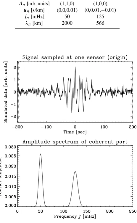
The model parameters are the periodsTnof the two plane waves, the slowness vectorsun, the amplitude vectorsAn, the widths τn of the Gaussian envelope function, and the noise amplitudeν. The wave parameter values used here are summarized in Table 1. The noise amplitude is set to the valueν=0.2.

The synthetic signal is assumed to be sampled in space at four locations, namely, at the origin of the cartesian coordi-nate system, and at three points on the coordicoordi-nate axes, each one at a distance of 200 km from the origin. The upper panel of Fig. 1 shows the generated signal at the sampling point in the origin. In the lower panel the amplitude spectrum of the coherent (noise-free) part of the model signal is displayed. As noted above, this amplitude spectrum does not depend on

Table 1. Wave parameter values for the synthetic signal consisting

of two planes waves in an isotropic noise background, see Eq. (36). Model parameters are the wave periodsTn, the slowness vectorsun, the amplitude vectorsAn, and the widthsτnof the Gaussian enve-lope function. The wave frequenciesfn=1/Tnand the wavelengths λn=Tn/|un|are added for convenience.

n=1 n=2

Tn[s] 20 8 τn[s] 60 40 An[arb. units] (1,1,0) (1,0,0)

un[s/km] (0,0,0.01) (0,0.01,−0.01) fn[mHz] 50 125

λn[km] 2000 566

Fig. 1. Demonstration of the wave surveyor technique. Upper

panel: Synthetic time series sampled at one of the four points in space. Lower panel: Amplitude spectrum of the coherent part of the model signal as a function of frequencyf=ω/2π.

The square modulus of the Fourier amplitude, i.e._| b(ω)|2 in our case, is a measure of the total signal power in the fre-quency domain. In minimum variance estimators like the wave telescope or thek-filtering method, such a power spec-trum estimate is used to identify the frequency bands with

Fig. 2. Demonstration of the wave surveyor technique. Eigenvalues

and trace of the CSD matrix as functions of frequencyf=ω/2π. First eigenvalue: solid line. Remaining eigenvalues: dotted lines. Trace of the CSD matrix: dashed line.

sufficient power to support waves. Since D

|b|2 E

= D

trace(bb†) E

=traceDbb†E=trace C, (39) this approach is equivalent to using the trace of the FSC ma-trix for inspecting the frequency domain. In the case of the CSD matrix M=M0C, its trace gives the total power spectral density.

In its principal axes system, the eigenvalues µ`=µ`(ω) of the CSD matrix reside on the diagonal, hence trace M=P

`µ`. As explained in Sect. 2.2 by means of the plane wave model, the wave signature shows up in the first mode, whereas the noisy part contributes equally to all eigen-values. Therefore, the eigenvalues of the CSD matrix effec-tively decompose the signal power into a number of modes of decreasing significance.

For the synthetic signal considered here, the eigenvalues and the trace of the CSD matrix are shown as functions of the frequencyf=ω/2πin Fig. 2. The peaks associated with the waves can be seen in both the trace of the CSD matrix and in its first eigenvalue (the remaining eigenvalues collect the contribution of the noisy part of the signal), however, the peaks in the first eigenvalue stand above the noise back-ground much more clearly than the peaks in the trace. In this sense, eigenstructure based methods like the wave surveyor technique can yield a better separation of the Fourier modes and the noise background in the frequency domain.

amplitude (polarization) vectora are computed directly as functions of frequency.

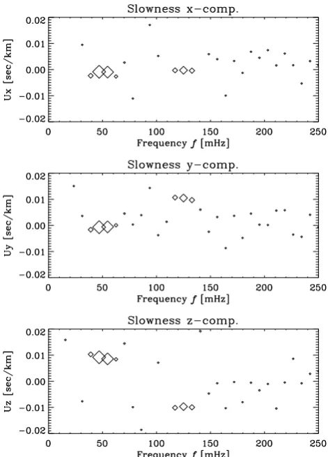
For the synthetic signal considered here, the components of the estimated slowness vector as functions of frequency f=ω/2πare shown in Fig. 3. At each frequency, the area of the diamond represents the power contained in the respective dominant mode as given by the largest eigenvalue. The sizes of the symbols are meant to serve as significance measures of the slowness vector estimates in the following way. In the frequency range outside the two bands supported by the plane waves where only the noise term contributes to the signal, there is relatively little power in the dominant modes, and the wave vector estimates cannot be considered meaningful. In the two frequency bands with significant wave power, the symbol sizes are larger, there is little scatter, and the results compare nicely with the parameters of the synthetic signals.

5 Application to Cluster FGM observations of fore-shock waves

In this section we show results of an application of the wave surveyor technique to magnetic field fluctuations recorded by the fluxgate magnetometer on board the four Cluster space-craft (Balogh et al., 2001). These observations were analysed already by Narita et al. (2007) using the well-established and thoroughly tested wave telescope analysis method (e.g. Neubauer and Glassmeier, 1990; Motschmann et al., 1996; Glassmeier et al., 2001; Narita et al., 2003) to study the dis-persion of foreshock waves. We may thus validate the wave surveyor approach by comparing our results with the findings of Narita et al. (2007).

The analysis example makes use only of one magnetic field component, namely, the Bz (northward) component in the GSE coordinate system. We thus follow the pro-cedure outlined in Sect. 3.1 for scalar data, see Eq. (28). The time interval of interest is 16 February 2002, 07:00– 07:45 UT, and it comprises Cluster observations of a rep-resentative case of foreshock waves. Narita et al. (2007) identified the whistler wave dispersion branch and demon-strated how it becomes Alfv´en wave dispersion (ω=kVA) at small wave numbers. Background plasma and magnetic field values were as follows: the mean magnetic field was pointing away from the sun (Bx=−5.6 nT, By=−1.4 nT, Bz=−1.4 nT in the GSE coordinate system), the plasma bulk velocity was almost 300 km/s (Vx=−300.7 km/s, Vy=24.3 km/s,Vz=2.8 km/s), and the ion density had the valuen=5.9 cm−3. The plasma velocity and density were provided by the ion measurements of the Cluster CIS-HIA instrument (R`eme et al., 2001).

The determination of the wave vectors further allows to transform the wave frequencies from the spacecraft frame (ωsc) into the plasma rest frame (hereafter, the rest frame,

ωre), a frame which is co-moving with the plasma bulk

ve-Fig. 3. Demonstration of the wave surveyor technique. The

com-ponents of the slowness vectoruare given as functions of the fre-quencyf=ω/2π. For each frequency, the area occupied by the plotting symbol is a measure of the signal power given by the largest eigenvalue. Only the frequency bands associated with the coherent part of the model signal yield significant power. The smaller dia-monds that show much scatter are associated with the contribution of the noise term to the model signal.

locity. This transformation is carried out using the Doppler relation:

ωre=ωsc−k·V, (40)

where V=(Vx, Vy, Vz)t denotes the plasma bulk velocity given above.

Figure 4 displays the dispersion relation, ωre=ωre(|k|),

Fig. 4. Experimental dispersion relation of the foreshock waves

(top) and propagation angles from the mean magnetic field direc-tion identified by the wave surveyor technique using Cluster mag-netic field data. The frequencies are represented in the plasma rest frame. The ion inertial scale and the ion cyclotron frequency are kin=0.011 rad/km andi=0.64 rad/s, respectively.

characteristic to the low frequency part of the whistler mode dispersion. The propagation direction is almost anti-parallel to the mean magnetic field, therefore the waves propagate intrinsically away from the bow shock.

In conclusion, the results obtained through the wave sur-veyor technique are fully consistent with the findings of Narita et al. (2007) using the wave telescope analysis.

6 Discussion

The wave surveyor technique is a direct method to estimate the parameters of a dominant plane wave in multipoint mea-surements. Isotropic white noise has no influence on the eigenvectors of the CSD matrix and hence does not change the estimated wave vectors or amplitude vectors. The pres-ence of other waves at the same frequency, however, may limit the applicability of the analysis method. Since their contributions to the total variance affect the eigenvalue dis-tribution of the CSD matrix, the eigenvalue ratios may be

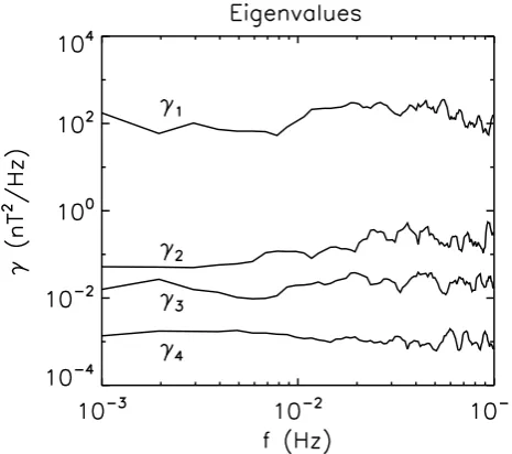
Fig. 5. Eigenvalues of the CSD matrix for the analysis example

presented in Sect. 5. The first eigenvalue is clearly much larger than the other eigenvalues throughout the whole frequency range which confirms that we are dealing with a single dominant mode in this case.

used to check the validity of the model assumptions. The single (dominant) plane wave model is expected to provide an appropriate characterization of the measured signal if the first eigenvalue proves to be much larger than the remaining ones.

The distribution of eigenvalues with frequency for the foreshock wave analysis event of Sect. 5 is shown in Fig. 5. Throughout the entire frequency range, the first eigenvalue is about three orders of magnitude larger than the other ones. Hence it is indeed quite safe to assume that the event is well characterized by the single (dominant) plane wave model. The practical significance of the eigenvalue ratios for the ro-bustness of the parameter estimation is shown also in Fig. 3 for the case of synthetic data: the frequency ranges where the first eigenvalues are large (corresponding to large plotting symbols) yield stable parameter estimates whereas the fre-quency ranges where noise dominates (small plotting sym-bols) exhibit a lot of scatter.

paper was meant to introduce the wave surveyor technique and to provide a proof of concept, we did not try to quantify threshold values neither for the angular mismatch quality in-dicator, nor for the eigenvalue ratios discussed above, and leave this issue for future studies.

Wave analysis techniques based on the cross spectral den-sity matrix implicitly concentrate on second order moments. In order to address more complex associations in multipoint measurements, the wave surveyor technique could be gen-eralized by means of a singular value decomposition (SVD) applied to theL×Ndata matrix b(ω)to yield

b=U·diag(√γ`)·V†. (41)

HereN is the number of ensembles (subintervals in time), diag(√γ`)denotes the diagonal matrix with elements

√ γ`, and the columns of U are identical with the eigenvectors of the FSC matrix. The matrix V, however, provides new infor-mation: it allows to address the variability in time and to test for stationarity.

We conclude this section with a few comments on how the eigenstructure decomposition of the FSC matrix can help to address selected aspects of the two main classes of wave identification methods discussed in the introduction. Pro-vided that we are dealing with a signal that can be described by the single (dominant) plane wave model, the linear parts of the sensor pair correlations that constitute the basis of the phase differencing approach are implicitly encoded in the phases of the first eigenvector. This follows from the rela-tionsh(k)∝cˆ1for the scalar case (see Sect. 3.1),h(k)∝5jcˆ1 for the case of vector data (see Sect. 3.2), and the definition of the vector functionh(k). As demonstrated by Dudok de Wit et al. (1995) for the case of two-point measurements, the phase differencing approach is suited to identify several waves at the same frequency whereas the wave surveyor tech-nique extracts the dominant wave only. Using four sensors instead of two allows to improve the effective signal-to-noise ratio, and in this case the inversion of the position tensor and thus the wave vector estimation in the wave surveyor technique can be carried out directly (see the Appendix) and with little effort. In the case of four-point phase differencing method, the improved signal-to-noise ratio goes along with a more involved reconstruction scheme (e.g. Matsui et al., 2007).

To gain additional insight into the performance of min-imum variance estimators, it is instructive to rewrite them using the eigendecomposition of the FSC matrix:

C=X `

γ`cˆ`cˆ†_`. (42) Since

ˆ

c`=C−1Cˆc`=C−1γ`cˆ`=γ`C−1cˆ`, (43) we obtain

C−1cˆ`=γ`−1cˆ` (44)

which means that thecˆ`, `=1, . . . , L,are eigenvectors also of the inverse matrix C−1_{, and the corresponding eigenvalues} areγ_`−1. Therefore, we can write

C−1= L X

`=1

γ<sub>`</sub>−1cˆ`cˆ†_`. (45)

For brevity, we consider the scalar case only. HenceL→S, `→σ, and the minimum variance estimator for the power spectral density estimate is given byP=(h†C−1h)−1 (e.g. Motschmann et al., 1995). The eigenstructure representation of C−1allows to rewriteP=P (ω,k)as follows:

P = h† " _S

X

σ=1

γ_σ−1cˆσcˆ†σ #

h† !−1

= S X

σ=1

γ_σ−1h†cˆσcˆ†σh† !−1

, (46)

therefore,

P (ω,k)= S X

σ=1

γ_σ−1|h†(k)ˆcσ(ω)|2 !−1

. (47)

For the single plane wave model,h(k)= √

Scˆ1which implies that h(k) ⊥ cˆσ for σ6=1, or, equivalently,h†(k)cˆσ=0 for the remaining eigenvectors cˆσ, σ=2, . . . , S. Furthermore, γ₁−1=(S|a|2+η2)−1, and the result is thus

P (ω,k)= |a|2+η2/S . (48) This has to be compared with the minimum value ofP in the case whenh(k0_{)lies in the noise subspace, i.e. the subspace}

spanned by the eigenvectorscˆσ, σ=2, . . . , S. Here we find P (ω,k0_)=η2_{/Sand thus}

Pmax

Pmin

=1+S|a| 2

η2 . (49)

Hence the resolving power of the scalar minimum variance estimator measured by this analytical expression increases (quadratically) with the signal-to-noise ratio (as expected). In practice, however, the numerical inversion of the CSD matrix C may cause problems if C is near singular which happens, e.g. in the case of a very large signal-to-noise ratio (|a|2η2/S) in the single plane wave model. In such a case one might be tempted to perform an inversion in the singular value sense and disregard the contributions of the smallest eigenvalues to obtain

C−1 =SVγ₁−1cˆ1cˆ†₁, (50) andPSV=γ1|h†cˆ1|−2. However, this would make the method completely useless. Although PSV(ω,k) gives the correct

would diverge towards infinity ifh(k0_{)was in the noise}

sub-space because thenh(k0_{) ⊥ cˆ}

1. This shows that and why minimum variance estimators require careful regularization schemes especially when the signal-to-noise ratio is very large.

7 Summary and conclusions

The wave surveyor technique introduced in this paper is de-signed to be a fast alternative to the existing wave analysis methods such as the wave telescope or the k-filtering ap-proach. The new technique was validated using a synthetic signal and also by means of Cluster magnetometer measure-ments. The model signal considered in Sect. 4 was processed within a few seconds on a standard PC, and the complete dispersion curve in Sect. 5 was generated in about a minute. The wave surveyor technique is most appropriate when the wavefield at each frequency contains a single dominant wave mode.

We concentrated on the case of four spacecraft where the wave vector can be expressed explicitly as a linear combina-tion of the reciprocal vectors of the tetrahedron. The wave surveyor approach, however, is not restricted to four sen-sors, and the more general case can be treated by means of Eq. (33). Applications of the generalized wave surveyor technique to missions with more than four spacecraft (like THEMIS), or even only three sensors (like several of the in-struments on the Cluster satellites) are planned to be topics of our future work.

Appendix A

Estimating the slowness vector from eigenvector phases We first note that the cost function in Sect. 3.1 can be written as

Q(k, φ)= S X

σ=1

θσ −ktrσ−φ 2

= S X

σ=1

(θσ)2+(ktrσ)2+φ2

−2θσktrσ−2θσφ+2ktrσφ

. (A1)

For notational convenience, and without loss of generality, we let the origin of the coordinate system coincide with the mean position of the sensor array. HenceP

σrσ=0 and 0 = 1

2 ∂ ∂φ

X

σ

(· · ·)2=Sφ−X σ

θσ

H⇒φ= 1 S

X

σ

θσ , (A2)

and 0=1

2 ∂ ∂k

X

σ

(· · ·)2=ktX

σ

rσrtσ − X

σ

θσrσ . (A3) This yields

k= X

σ

r_σrt_σ !−1

X

σ

θσrσ . (A4)

This result is still general with respect to the number of sen-sorsS in the array as long as the position tensorP

σrσrtσ is regular. In the singular or near-singular case, the exact inverse of this tensor may be replaced by the pseudo-inverse. ESA’s Cluster mission consists of four spacecraft, hence S=4, and the inverse of the position tensor can be expressed through the reciprocal vectorsκσ of the Cluster tetrahedron as follows:

X

σ

rσrtσ !−1

=X τ

κτκtτ (A5)

(for a proof see Chanteur and Harvey, 1998). For a thorough discussion of the reciprocal vector concept in the context of the Cluster mission, the reader is referred to Chanteur (1998). The reciprocal vector of spacecraft 1, for example, is given as

κ1=

r23×r24

r21·(r23×r24)

(A6) where rij denotes the position vector pointing from the spacecraftj toi, i.e.rij=rj−ri. The other three recipro-cal vectors,κ2,κ3, andκ4, are obtained in the same fashion by shifting the indices(1,2,3,4)cyclically into(2,3,4,1), (3,4,1,2), and(4,1,2,3), respectively.

Inserting Eq. (A5) into Eq. (A4) allows to express the wave vectorkof the plane wave in terms of the eigenvector phases θσ=θσ(ω), the spacecraft positionsrσ relative to their mean location, and the reciprocal vectorskσ as follows:

k=X

τ

κτκtτ X

σ

θσrσ = X

σ,τ

θσκτκtτrσ . (A7)

Since κt_τrσ=δτ,σ−1/4 (Eq. 15.1 in Chanteur and Harvey, 1998) andP

σκσ=0 (Eq. 14.10 in Chanteur, 1998), we fi-nally obtain

ωu=k=X σ

θσκσ (A8)

References

Balikhin, M. A. and Gedalin, M. E.: Comparative analysis of dif-ferent methods for distinguishing temporal and spatial variations, in: ESA WPP-047: Proc. of Start Conf., Aussois, France, pp. 183–187, 1993.

Balogh, A., Carr, C. M., Na, M. H. A., Dunlop, M. W., Beek, T. J., Brown, P., Fornac¸on, K.-H., Georgescu, E., Glassmeier, K.-H., Harris, J., Musmann, G., Oddy, T., and Schwingenschuh, K.: The Cluster magnetic field investigation: overview of in-flight performance and initial results, Ann. Geophys., 19, 1207–1217, 2001,

http://www.ann-geophys.net/19/1207/2001/.

Capon, J.: High Resolution Frequency-Wavenumber Spectrum Analysis, in: Proc. IEEE, 57, 1408–1418, 1969.

Capon, J., Greenfield, R. J., and Kolker, R. J.: Multidimensional maximum-likelihood processing of a large aperture seismic ar-ray, in: Proc. IEEE, 55, 192–213, 1967.

Chanteur, G.: Spatial Interpolation for Four Spacecraft: The-ory, in: Analysis Methods for Multi-Spacecraft Data, edited by: Paschmann, G. and Daly, P., pp. 371–393, ISSI/ESA, 1998. Chanteur, G. and Harvey, C. C.: Spatial Interpolation for Four

Spacecraft: Application to Magnetic Gradients, in: Analysis Methods for Multi-Spacecraft Data, edited by: Paschmann, G. and Daly, P., pp. 349–369, ISSI/ESA, 1998.

Constantinescu, O. D., Glassmeier, K.-H., D´ecr´eau, P. M. E., Fr¨anz, M., and Fornac¸on, K.-H.: Low frequency wave sources in the outer magnetosphere, magnetosheath, and near Earth solar wind, Ann. Geophys., 25, 2217–2228, 2007,

http://www.ann-geophys.net/25/2217/2007/.

Cox, H.: Resolving power and mismatch of optimum array proces-sors, J. Acoust. Soc. Am., 54, 771–785, 1973.

Dudok de Wit, T., Krasnosel’skikh, V. V., Bale, S. D., Dunlop, M. W., L¨uhr, H., Schwartz, S. J., and Woolliscroft, L. J. C.: De-termination of dispersion relations in quasi-stationary plasma tur-bulence using dual satellite data, Geophys. Res. Lett., 22, 2653– 2656, doi:10.1029/95GL02543, 1995.

Dunlop, M. W., Southwood, D. J., Glassmeier, K.-H., and Neubauer, F. M.: Analysis of multipoint magnetometer data, Adv. Space Res., 8, 273–1177, 1988.

Eriksson, A. I.: Spectral Analysis, in: Analysis Methods for Multi-Spacecraft Data, edited by: Paschmann, G. and Daly, P., pp. 5– 42, ISSI/ESA, 1998.

Glassmeier, K.-H., Motschmann, U., Dunlop, M., Balogh, A., Acuna, M. H., Carr, C., Musmann, G., Fornacon, K.-H., Schweda, K., Vogt, J., Georgescu, E., and Buchert, S.: Cluster as a wave telescope – first results from the fluxgate magnetome-ter, Ann. Geophys., 19, 1439–1447, 2001,

http://www.ann-geophys.net/19/1439/2001/.

Matsui, H., Puhl-Quinn, P. A., Torbert, R. B., Baumjohann, W., Far-rugia, C. J., Mouikis, C. G., Lucek, E. A., D´ecr´eau, P. M. E., and Paschmann, G.: Cluster observations of broadband ULF waves near the dayside polar cap boundary: Two detailed multi-instrument event studies, J. Geophys. Res., 112, A07 218, doi: 10.1029/2007JA012251, 2007.

Motschmann, U., Woodward, T. I., Glassmeier, K.-H., and Dunlop, M. W.: Array Signal Processing Techniques, in: ESA SP-371: Proceedings of the Cluster Workshops, Data Analysis Tools and Physical Measurements and Mission-Oriented Theory, pp. 79– 86, 1995.

Motschmann, U., Woodward, T. I., Glassmeier, K. H., and South-wood, D. J.: Wave field analysis by magnetic measurements at satellite arrays: generalized minimum variance analysis, Adv. Space Res., 18, 315–319, 1996.

Narita, Y. and Glassmeier, K.-H.: Dispersion analysis of low-frequency waves through the terrestrial bow shock, J. Geophys. Res., 110, 12 215, doi:10.1029/2005JA011256, 2005.

Narita, Y., Glassmeier, K.-H., Sch¨afer, S., Motschmann, U., Sauer, K., Dandouras, I., Fornac¸on, K.-H., Georgescu, E., and R`eme, H.: Dispersion analysis of ULF waves in the foreshock using cluster data and the wave telescope technique, Geophys. Res. Lett., 30, 43–1, doi:10.1029/2003GL017432, 2003.

Narita, Y., Glassmeier, K.-H., and Treumann, R. A.: Wave-Number Spectra and Intermittency in the Terrestrial Foreshock Region, Phys. Rev. Lett., 97, 191 101, doi:10.1103/PhysRevLett. 97.191101, 2006.

Narita, Y., Glassmeier, K.-H., Fr¨anz, M., Nariyuki, Y., and Hada, T.: Observations of linear and nonlinear processes in the foreshock wave evolution, Nonlin. Processes Geophys., 14, 361–371, 2007, http://www.nonlin-processes-geophys.net/14/361/2007/. Neubauer, F. M. and Glassmeier, K.-H.: Use of an array of satellites

as a wave telescope, J. Geophys. Res., 95, 19 115–19 122, 1990. Pillai, S. U.: Array signal processing, Springer, New York, 1989. Pincon, J. L. and Lefeuvre, F.: Local characterization of

homoge-neous turbulence in a space plasma from simultahomoge-neous measure-ments of field components at several points in space, J. Geophys. Res., 96, 1789–1802, 1991.

Pincon, J. L. and Lefeuvre, F.: The application of the generalized Capon method to the analysis of a turbulent field in space plasma - Experimental constraints, J. Atmos. Terr. Phys., 54, 1237–1247, 1992.

Pincon, J. L. and Motschmann, U.: Multi-Spacecraft Filtering: General Framework, in: Analysis Methods for Multi-Spacecraft Data, edited by: Paschmann, G. and Daly, P., pp. 65–78, ISSI/ESA, 1998.

R`eme, H., Aoustin, C., Bosques, J. M., Dandouras, I., et al.: First multispacecraft ion measurements in and near the Earth’s mag-netosphere with the identical Cluster ion spectrometry (CIS) ex-periment, Ann. Geophys., 19, 1303–1354, 2001,

http://www.ann-geophys.net/19/1303/2001/.

Sahraoui, F., Pinc¸on, J. L., Belmont, G., Rezeau, L., Cornilleau-Wehrlin, N., Robert, P., Mellul, L., Bosqued, J. M., Balogh, A., Canu, P., and Chanteur, G.: ULF wave identification in the mag-netosheath: The k-filtering technique applied to Cluster II data, J. Geophys. Res., 108, 1–1, 2003.

Sahraoui, F., Belmont, G., Rezeau, L., Cornilleau-Wehrlin, N., Pinc¸on, J. L., and Balogh, A.: Anisotropic Turbulent Spectra in the Terrestrial Magnetosheath as Seen by the Cluster Space-craft, Phys. Rev. Lett., 96, 075 002, doi:10.1103/PhysRevLett. 96.075002, 2006.

Samson, J. C.: Pure states, polarized waves, and principal compo-nents in the spectra of multiple, geophysical time-series, Geo-phys. J. R. Astr. Soc., 72, 647–664, 1983.

Samson, J. C. and Olsen, J. V.: Some comments on the descriptions of the polarization states of waves, Geophys. J. R. Astr. Soc., 61, 115–129, 1980.

Geophys. Res., 95, 7693–7709, 1990.

Santol´ık, O., Parrot, M., and Lefeuvre, F.: Singular value decom-position methods for wave propagation analysis, Radio Science, 38, 10–1, doi:10.1029/2000RS002523, 2003.

Schmidt, R. O.: Multiple emitter location and signal parameter esti-mation, in: Proc. RADC Spectral Est. Workshop, Oct. 1979, pp. 243–258, pp. 243–258, 1979.

Schmidt, R. O.: A signal subspace approach to emitter location and spectral estimation, Ph.D. Dissertation, Stanford Univ., Stanford, CA, 1981.

Storey, L. R. O.: The measurement of wave distribution functions, in: Modern Radio Science 1999, edited by: Stuchly, M. A., pp. 249–271, Oxford University Press, 1999.

Walker, S., Sahraoui, F., Balikhin, M., Belmont, G., Pinc¸on, J., Rezeau, L., Alleyne, H., Cornilleau-Wehrlin, N., and Andr´e, M.: A comparison of wave mode identification techniques, Ann. Geophys., 22, 3021–3032, 2004,