Ann. Geophys., 32, 563–569, 2014 www.ann-geophys.net/32/563/2014/ doi:10.5194/angeo-32-563-2014
© Author(s) 2014. CC Attribution 3.0 License.
A method to identify aperiodic disturbances in the ionosphere
J.-S. Wang1, Z. Chen2,1, and C.-M. Huang2
1National Center for Space Weather, China Meteorological Administration, Beijing 100081, China 2School of Electronic Information, Wuhan University, Hubei 430072, China
Correspondence to: J.-S. Wang ([email protected])
Received: 24 October 2013 – Revised: 20 March 2014 – Accepted: 21 April 2014 – Published: 26 May 2014
Abstract. In this paper, variations in the ionospheric F2 layer’s critical frequency are decomposed into their peri-odic and aperiperi-odic components. The latter include distur-bances caused both by geophysical impacts on the iono-sphere and random noise. The spectral whitening method (SWM), a signal-processing technique used in statistical esti-mation and/or detection, was used to identify aperiodic com-ponents in the ionosphere. The whitening algorithm adopted herein is used to divide the Fourier transform of the ob-served data series by a real envelope function. As a re-sult, periodic components are suppressed and aperiodic com-ponents emerge as the dominant contributors. Application to a synthetic data set based on significant simulated peri-odic features of ionospheric observations containing artifi-cial (and, hence, controllable) disturbances was used to val-idate the SWM for identification of aperiodic components. Although the random noise was somewhat enhanced by post-processing, the artificial disturbances could still be clearly identified. The SWM was then applied to real ionospheric ob-servations. It was found to be more sensitive than the often-used monthly median method to identify geomagnetic ef-fects. In addition, disturbances detected by the SWM were characterized by a Gaussian-type probability density func-tion over all timescales, which further simplifies statistical analysis and suggests that the disturbances thus identified can be compared regardless of timescale.
Keywords. Ionosphere (ionospheric disturbances)
1 Introduction
The variability of the critical frequency of the ionospheric F2 layer (foF2) is a proxy for the complex behavior of the ionosphere. In the frequency domain, periodicity is the most
significant feature in the foF2’s power spectrum, as indicated by the vertical dash-dotted lines in Fig. 1a. The black curve is similar to that in Fig. 1 of Liu et al. (2011), based on observa-tions at Canberra (149.0◦E, 35.3◦S) obtained between 1950 and 2007, and with a time resolution of one hour. In general, the intensity of the power spectrum increases with decreasing frequency. However, aperiodic variations do not exhibit any prevailing frequency. They do not show any periodicity, and they cannot be read off directly from the frequency domain. Unlike periodic signals, which are easy to both distinguish (e.g., through filtering) and model (e.g., Zhao et al., 2005), aperiodic variations in the ionosphere are usually discussed case by case; in addition, they are difficult to distinguish au-tomatically. This difficulty has its origin in the complexity of the ionosphere’s behavior, which is modulated by solar ra-diation, the solar wind, and its geomagnetic consequences, the neutral atmosphere, as well as by electrodynamical pro-cesses (Rishbeth and Mendillo, 2001). These modulations re-veal themselves partially as periodic signals and also as ape-riodic disturbances in the ionosphere.
564 J.-S. Wang et al.: A method to identify aperiodic disturbances in the ionosphere 329
330
Fig. 1. (a) Power spectrum of the foF2 at Canberra during the period 1950‒2007 (black).
331
Significant periods are indicated by vertical dash-dotted lines. The flattened spectrum is shown in 332
grey; the power intensities at all frequencies have been suppressed to below a given value, so that 333
no single frequency is dominant. (b) Spectrum (black) of a simulated dataset and its flattened 334
spectrum (grey). 335
336
337
Figure 1. (a) Power spectrum of the foF2 at Canberra during the
period 1950–2007 (black). Significant periods are indicated by ver-tical dash-dotted lines. The flattened spectrum is shown in grey; the power intensities at all frequencies have been suppressed to below a given value, so that no single frequency is dominant. (b) Spectrum (black) of a simulated data set and its flattened spectrum (grey).
as the background, to random noise as noise, and to other aperiodic components as aperiodic disturbances.
The spectral whitening method (SWM) is a technique of-ten used for statistical estimation and detection. It is useful for either decorrelating a data sequence or controlling the spectral shape (Eldar and Oppenheim, 2003). The SWM is adopted to remove the periodic components from the foF2 variations by flattening the Fourier spectrum and therefore to identify the aperiodic components (particularly the aperiodic disturbances).
2 Methodology
To illustrate this SWM approach and to test its validity, a sim-ulated signal series,g(t )(where timetis expressed in hours; Fig. 2a), was generated from (1) all of the major periodic components highlighted in Fig. 1a; and (2) a total of 100 (al-though this number can be changed arbitrarily) segments of artificial disturbances,gd, of random amplitudes and random durations (but less than 72 h), consistent with typical iono-spheric disturbances caused by geomagnetic storms (cf. Zhao
et al., 2008, and references therein), distributed randomly in time and connected by random noise (Fig. 2b). The data set length, the time period, and even the data loss characteris-tics were also set to be identical to those pertaining to the Canberra foF2 data set. Thus,
g(t )=
7
X
i=0
Aicos(2π ξit+φi)+gd, (1)
whereξi represents the ith frequency of the main periodic components indicated by the vertical dash-dotted line in Fig. 1a (iruns from 0 to 7, where 0 represents the DC com-ponent);Ai and φi are the amplitude and phase of theith periodic component, whereφi is set randomly.Ai is initially set by reference to the Fourier transform of the Canberra foF2 data set. Due to the randomness ofφiandgd, adjustments to Ai were applied to improve the similarity between the spec-trums ofg(t )(Fig. 1b) and the Canberra foF2 (Fig. 1a). The spikes at higher frequencies than that of the terdiurnal com-ponent in Fig. 1a were not included in the synthetic data, as these components are the high-frequency harmonics of the diurnal variation, which are usually not considered. It ap-pears that aperiodic disturbances can be distinguished only when they are not buried in periodic signals. It is impossible, and (fortunately) unnecessary, to simultaneously filter out all periodic components. It is sufficient to detect aperiodic com-ponents under conditions where every periodic component has been reduced to, or below, the level of the aperiodic com-ponents. That is, all discernible spikes, humps, or slopes in the spectrum (Fig. 1) related to periodic components need to be polished, so that there is no higher power intensity at any frequency. Visually, this corresponds to a power spec-trum that is flattened.
Spectral flattening can be achieved through application of the SWM, although the whitening algorithm is not unique (Eldar and Oppenheim, 2003). In this paper, we whiten the foF2 data sequence by dividing the Fourier transform of the observed data series by a real envelope function.
Considering a transformation fromg(t )togd0(t ), gd∗(t )=
R+∞ −∞ [
R+∞ −∞g(t )·e
−2π it ξdt] · P0 Penv(ξ )·e
2π it ξdξ (2) and
gd0(tm)=13 2
P
j=0
g∗d(tm+j−1) , (3)
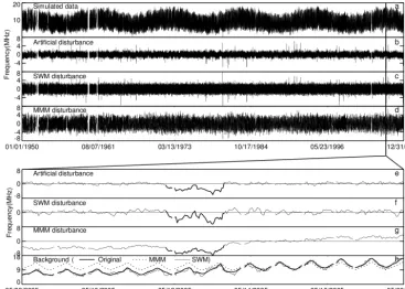
[image:2.612.46.286.65.355.2]J.-S. Wang et al.: A method to identify aperiodic disturbances in the ionosphere 565
338
Fig. 2. (a) Simulated time series. (b) Artificial disturbances of random amplitudes and random 339
durations distributed randomly in time with additional random noise. (c) Spectrum of the flattened 340
signal. (d) Disturbances identified by the MMM. (e), (f), and (g) Magnified period corresponding 341
to panels (b), (c), and (d), respectively. (h) Comparison of the original, SWM, and MMM 342
backgrounds. 343
344
345
346
Figure 2. (a) Simulated time series. (b) Artificial disturbances of random amplitudes and random durations distributed randomly in time
with additional random noise. (c) Spectrum of the flattened signal. (d) Disturbances identified by the MMM (monthly median method).
(e), (f), and (g) Magnified period corresponding to panels (b), (c), and (d), respectively. (h) Comparison of the original, SWM, and MMM
backgrounds.
i.e., it is the mode ofPenv(ξ ). The transformation above con-sists of four steps. (1) A Fourier transformation, shown as the bracketed part in Eq. (2), is applied to the original data, while a periodic extension is imposed on the original time series to avoid boundary effects affecting the transformation (Gonzalez-Velasco, 1995). (2) The Fourier power spectrum is divided by its upper envelope Penv(ξ ), so that the maxi-mum intensity becomes unity. The spectrum is thus flattened and displays the spectral form of white noise (i.e., it has been whitened). As the aperiodic components are, in fact, not discernible in the spectrum, they are hardly affected by the whitening process. (3) The whitened spectrum is multi-plied byP0to ensure that the most commonly occurring val-ues of the spectrum’s intensity remain the same before and after whitening. In other words, most components approxi-mately retain the same amplitudes before and after the trans-formation. The spectrum thus whitened is shown in grey in Fig. 1b. (4) An inverse Fourier transformation is applied to the whitened spectrum and a new time series, g∗d(t ), is de-rived. The whitening process degrades the periodic compo-nents to noise and, therefore, additional random dithers are introduced. To reduce the enhanced noise, a three-point run-ning average is applied to smoothgd∗(t )and the final result, gd0(t ), is obtained (Fig. 2c). It is easily found thatgd0(t )can reproduce most features of gd(t )(compare Fig. 2b and c, as well as e and f), and the correlation coefficient of g0d(t )
andgdattains values of up to 0.89, which is an improvement over the correlation coefficient found below for the monthly median method (MMM). The major difference is the rela-tively larger amplitude of the irregular dithers ingd0(t ). The derived background, i.e.,g(t )−gd0(t ), is nearly the same as g(t )−gd(t ), except for small-amplitude random deviations (Fig. 2h). Thus, the SWM introduced here is capable of iden-tifying aperiodic components among periodic signals.
[image:3.612.114.481.68.330.2]566 J.-S. Wang et al.: A method to identify aperiodic disturbances in the ionosphere
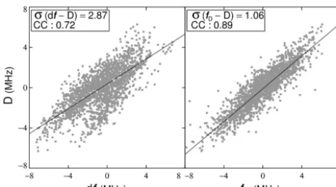
Figure 3. Comparison of the original disturbance (D) and the MMM
disturbance (df ), as well as of D and the SWM disturbance (fD).
σ(df–D) andσ (fD–D) are the variances of df–D andfD–D,
re-spectively. CC: correlation coefficient of the parameters on both axes.
time window chosen covers the month prior to the observa-tion time (i.e., we use a backward-running median) so as to simulate real-time data processing. The MMM is a good ap-proach when attempting to distinguish periodic components from aperiodic disturbances when the ionosphere is suffi-ciently stable such that all foF2 values are very close to the median value. However, its efficacy will decrease when day-to-day ionospheric variations are significant (Fig. 2h). For the simulated data set, the MMM can detect man-made pertur-bations, but there is still a systematic offset, which is caused by the differences between the monthly median value and the real background (Fig. 2g). For the entire synthetic data set, the MMM is used to achieve a correlation coefficient of 0.71 between the original and derived disturbances. This is good but of lower significance than the SWM’s correlation coefficient of 0.89. Moreover, the variance of the deviation between the original and derived disturbances is 1.06 as de-rived using the SWM, which is much lower than the MMM-based value of 2.88 (Fig. 3). In fact, if we shift the median widow of the MMM day by day from one month before the observation time to one month after, the correlation coeffi-cient varies from 0.57 to 0.73. This indicates that the SWM can reproduce the aperiodic disturbances more precisely and is, therefore, generally better than the MMM at identifying aperiodic disturbances from periodic components.
In the context of other Fourier-transformation filtering pro-cesses, such as band-pass filtering, the transformation ker-nel is a window function that is used to strongly constrain the intensities around the frequencies of interest (Gonzalez-Velasco, 1995). To identify aperiodic components, it is the-oretically necessary to simultaneously filter out all periodic signals, which is normally impossible unless the frequencies subject to filtering are all known and discrete. However, it is not necessary to do so, because if all periodic components are reduced to, or below, the level of the aperiodic compo-nents, the latter are easily discernible, and this is the function
of our SWM application. The SWM can be considered to be a type of Fourier-transformation filter with a special kernel, Penv/P0(ξ ). This kernel suppresses all known and unknown periodic components with power intensities in excess ofP0 to the level ofP0, so that they are rendered unimportant and other components (i.e., the aperiodic disturbances and noise) emerge. Meanwhile, the most common spectrum intensity (P0)is unchanged, so that the signals before and after pro-cessing, i.e., the original data and aperiodic disturbances (as well as the noise) are consistent in amplitude. However, note that the suppressed periodic features have been reduced and have become part of the noise, thus contributing to the ir-regular variations. This implies that the SWM is not suitable for the detection of disturbances at frequencies around the original sampling frequency. Meanwhile, the SWM cannot deal with perturbations characterized by durations that are similar to the observation duration. Despite these shortcom-ings, successful application to the synthetic data set validates the SWM’s efficacy in distinguishing aperiodic disturbances from periodic components.
Note that the MMM is often used, but it is not always the most appropriate of the median or mean methods that use different window widths to distinguish between the back-ground and perturbations. A specific window width set by the requirements pertaining to the issue under investigation usually leads to better results than a fixed width of 1 month. However, this means that one must determine the most suit-able width case by case. As shown here, the SWM is question independent, and can be applied universally to any time se-quence to which a Fourier transformation can be applied.
3 Application to the ionosphere
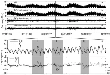
We next applied the SWM to the Canberra foF2 data set (1950–2007). The original foF2 and the SWM-derived ape-riodic disturbances (denotedfD), as well as the background variation,fB=foF2 −fD, are compared in Fig. 4. As ex-pected,fB represents the general foF2 variation, while fD (which varies around zero) demonstrates the foF2 fluctua-tions. As all periodic components have been reduced to such a level that no specific frequency is significantly stronger than any other, the significant fluctuations infDare related to the aperiodic components, as suggested by the synthetic data. Given the proven success of the SWM in identifying aperiodic disturbances, it is interesting to explore the addi-tional information the SWM can offer compared to other methods such as the MMM. We denote the monthly me-dian of the foF2 asfr and define df =foF2 −fr. To sim-plify the descriptions, the backgrounds and disturbances de-rived on the basis of the SWM and MMM are referred to as SWM background (fB), SWM disturbance (fD), MMM background (fr), and MMM disturbance (df ).
J.-S. Wang et al.: A method to identify aperiodic disturbances in the ionosphere 567 Fig. 3. Comparison of the original disturbance (D) and the MMM-disturbance (df), as well as of D
347
and the SWM-disturbance (fD). σ(df–D) and σ(fD–D) are the variances of df–D and fD–D, 348
respectively. CC: correlation coefficient of the parameters on both axes. 349
350
351
Fig. 4. (a) Observed foF2 at Canberra for the period 1950‒2007. (b) Background derived using 352
the SWM. (c) Disturbance derived based on application of the SWM. (d) Disturbance derived 353
using the MMM. A single solar-rotation period (27 days) was used to investigate the detailed 354
features of the observed and derived parameters in (e) and (f). The Dst index is also plotted as the 355
thick solid curve in (f). 356
357
Figure 4. (a) Observed foF2 at Canberra for the period 1950–2007. (b) Background derived using the SWM. (c) Disturbance derived based
on application of the SWM. (d) Disturbance derived using the MMM. A single solar-rotation period (27 days) was used to investigate the detailed features of the observed and derived parameters in (e) and (f). The Dst index is also plotted as the thick solid curve in (f).
apparent when the figure is enlarged (Fig. 4e and f). As the MMM background is composed of the median foF2 val-ues measured during the month before the reference date, it is stable and smooth, i.e., similar to that in the simula-tion, although foF2 variations occur much more frequently than their simulated counterparts. In comparison, the SWM background shows more features than either the MMM back-ground or the simulated SWM results (Fig. 2h). These differ-ences are reflected in the behavior of the perturbations. Dur-ing the shaded periods in Fig. 4e and f, the periods when ei-therfrorfBdeviate significantly from the observed foF2 are reflected by the corresponding trends infD and df, respec-tively. During Period (I),fDand df are similar, but for Peri-ods (II) and (III),fDis larger than df. The Dst index (Fig. 4f, thick solid curve) indicates that during Period (II) a geomag-netic storm occurred. The drop in the foF2 is the ionospheric response to the storm. The change in fD (=foF2 −fB)is more significant than that in df (=foF2−fr; Fig. 4f) or, equivalently, fD is more sensitive to external disturbances than df. As geomagnetic storms mainly contribute to ape-riodic perturbations in the foF2 (in addition to contributing weak, recurrent components), the period of solar rotation is only marginally discernible in the foF2 power spectrum. The significance of the period of solar rotation is much lower than that of other spectra (Fig. 1a). In addition, the SWM can sup-press the narrow hump around the period of solar rotation in the spectrum and blur the imprints of recurrent geomagnetic
358
Fig. 5. Difference between the maximum absolute values of df and fD (i.e., fDm‒dfm) compared 359
with the minimum Dst (Dstm) during periods when Dst is continuously less than –20 nT for at least 360
24 hours. Negative and positive disturbances according to fD are represented by black and grey 361
dots, respectively. 362
363
364
365
Figure 5. Difference between the maximum absolute values of
dfand fD (i.e., fDm–dfm) compared with the minimum Dst
(Dstm)during periods when Dst is continuously less than−20 nT
for at least 24 h. Negative and positive disturbances according tofD
are represented by black and grey dots, respectively.
storms (Kamide and Chian, 2007), but it leaves that of aperi-odic storms in the SWM disturbance.
[image:5.612.115.484.66.318.2] [image:5.612.325.527.383.549.2]568 J.-S. Wang et al.: A method to identify aperiodic disturbances in the ionosphere
Table 1. Difference betweenfDmand dfmunder different geomagnetic conditions.
Dstm −20 to−50 nT −50 to−100 nT −100 to−150 nT <−150 nT Total
|fDm|>|dfm| 76.6 % 74.4 % 64.1 % 70.1 % 71.9 %
fDm<0 46.1 % 48.4 % 55.1 % 74.8 % 54.2 %
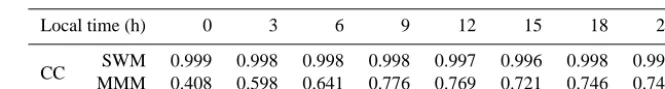
Table 2. Correlation coefficients (CCs) of the PDFs of SWM/MMM-derived disturbances and their best fits to a Gaussian function.
Local time (h) 0 3 6 9 12 15 18 21
CC SWM 0.999 0.998 0.998 0.998 0.997 0.996 0.998 0.999 MMM 0.408 0.598 0.641 0.776 0.769 0.721 0.746 0.749
each represented by their minimum Dst value, Dstm. Over a certain GAP, each interval where fD was continuously greater/less than zero for at least six hours (a criterion cho-sen to match the time criterion for ionospheric storms, e.g., Matuura, 1972; Fuller-Rowell et al., 1994) was recognized as an ionospheric disturbance. All disturbances occurring during the same GAP were compared, and thefD with the maximum absolute value is referred to as fDm. The iono-spheric disturbance during this GAP was recorded as a pos-itive or negative disturbance iffDm>0 orfDm<0, respec-tively. The corresponding df with the maximum absolute value during the same GAP is denoted dfm. The difference between dfmandfDm(i.e.,fDm−dfm)is plotted as a func-tion of the corresponding Dstmin Fig. 5. Positive (negative) disturbances are plotted as grey (black) dots. In nearly 72 % of cases, the amplitude of fDm is greater than that of dfm (i.e.,fDm>dfmfor positive cases andfDm<dfmfor nega-tive cases) during GAPs (Fig. 5; Table 1). The difference can be up to 5 MHz, i.e., approximately 1/3 of the maximum ob-served foF2 (ca. 15 MHz). Obviously, the SWM disturbance is more sensitive to strong geomagnetic activity. Figure 5 shows that negative ionospheric disturbances generally occur more often than positive perturbations. For Dst<−100 nT, the stronger the geomagnetic activity is, the more negative the ionospheric disturbances become (Fig. 5; Table 1).
This result is in accordance with previously obtained sta-tistical conclusions about positive and negative phases of ionospheric storms in similar regions (Prölss, 1993, 1995; Tsagouri, 2000). It is not strange that the aperiodic distur-bances discussed here share some features with ionospheric storms, because such storms are, in fact, intense disturbances (e.g., Rush, 1976).
4 Discussion
The MMM, which blurs the day-to-day differences within a given month, is in fact a high-stop filtering approach. The SWM, on the other hand, does not cause any frequency to become notably stronger than any other frequency, so that all features with distinct periodic components will be retained in
the SWM background and, hence, periodic components can-not be found in the SWM disturbance. Equivalently, there is no typical frequency in the SWM disturbance. The fact that the SWM disturbance is not associated with any typical frequency results in some interesting characteristics in the probability domain. The probability density function (PDF; Billingsley, 1979) of the SWM disturbances at different local times was compared with its best fit to a Gaussian function, and their correlation coefficient was always close to unity (Table 2). This indicates that the SWM disturbance’s PDF is Gaussian, which is due to the spectral-whitening process. For comparison, the PDF of the MMM disturbance differs signif-icantly from a Gaussian distribution and varies with observa-tion time (Table 2).
[image:6.612.127.460.168.212.2]J.-S. Wang et al.: A method to identify aperiodic disturbances in the ionosphere 569
5 Conclusions
In this paper, the SWM was introduced to identify iono-spheric aperiodic disturbances. Although the SWM could en-hance the noise and is unsuitable for the identification of perturbations characterized by very short (i.e., close to the sampling period) or very long (i.e., comparable with the data set length) timescales, its validation based on application of the SWM to a synthetic data set (which simulated the main features of ionosphere observations) demonstrates that the SWM can identify aperiodic disturbances in the ionosphere. Similarly to the commonly used MMM, the SWM can be ap-plied to all ionospheric data sets, but it yields a better back-ground than the MMM. The main advantage of this char-acteristic is that the SWM-derived disturbances in the iono-sphere are more sensitive to external geophysical perturba-tions than their MMM-derived counterparts. Meanwhile, dis-turbances identified by the SWM have a Gaussian-type PDF, which not only simplifies further statistical analysis by virtue of the well-known characteristics of Gaussian-type PDFs, but also simplifies comparisons of the disturbances at different times, regardless of the underlying physical processes. This comparability at different times offers the possibility to de-fine an ionospheric disturbance index in future studies.
Acknowledgements. We thank the IPS and the World Data Center
for Geomagnetism for making their data public. This research was funded by the National Natural Science Foundation of China (grant 40931056).
Topical Editor K. Hosokawa thanks P. Wilkinson and R. Cosgrove for their help in evaluating this paper.
References
Billingsley, P.: Probability and Measure, John Wiley and Sons, New York, Toronto, London 1979.
Bruce, J. W. and Giblin, P. J.: Curves and Singularities, Cambridge University Press, 2nd Edn., 99–131, ISBN 0-521-42999-4, 1992. Eldar, Y. C. and Oppenheim, A. V.: MMSE whitening and subspace whitening, IEEE Trans. Inform. Theory, 49, 1846–1851, 2003. Fuller-Rowell, T. J., Codrescu, M. V., Moffett, R. J., and
Quegan, S.: Response of the thermosphere and ionosphere to geomagnetic storms, J. Geophys. Res., 99, 3893–3914, doi:10.1029/93JA02015, 1994.
Gonzalez-Velasco, E. A.: Fourier Analysis and Boundary Value Problems, University of Massachusetts Press, 1995.
Kagan, A. and Shepp, L. A.: Why the variance?, Stat. Probabil. Lett., 38, 329–333, doi:10.1016/S0167-7152(98)00041-8, 1998. Kamide, Y. and Chian, A. C.-L.: Handbook of the Solar-Terrestrial
Environment, Springer-Verlag Berlin Heidelberg, 2007. Liu, L., Wan, W., Chen, Y., and Le, H.: Solar activity effects of
the ionosphere: A brief review, Chin. Sci. Bull., 56, 1202–1211, doi:10.1007/s11434-010-4226-9, 2011.
Matuura, N.: Theoretical models of ionospheric storms, Space Sci. Rev., 13, 124–189, 1972.
Perrone, L. and Di Franceschi, G.: Solar, Ionospheric, and Geomag-netic Indices, Annali di Geofisica, 41, 843–855, 1998.
Piggott, W. R. and Rawer, K. (Eds.): URSI Handbook of Ionogram Interpretation and Reduction, 2nd Edn., Report UAG-23,WDC-A for STP, NOUAG-23,WDC-AUAG-23,WDC-A, Boulder, Colorado, 1972.
Prölss, G. W.: On explaining the local time variation of ionospheric storm effects, Ann. Geophys., 11, 1–9, 1993,
http://www.ann-geophys.net/11/1/1993/.
Prölss, G. W.: Ionospheric F-region storms, in Hand-book of Atmo-spheric Electrodynamics, CRC Press, Boca Raton, Fla., 2, 195– 248, 1995.
Rice, J. A.: Mathematical statistics and data analysis, Duxbury Press, 2nd Edn., 163-164,ISBN 0-534-20934-3, 1995.
Rishbeth, H. and Mendillo, M.: Patterns of ionospheric variability, J. Atmos. Sol. Terr. Phys., 63, 1661–1680, 2001.
Rush, C. M.: An ionospheric observation network for use in short-term propagation predictions, Telecommunication J., 43, 544– 549, 1976.
Tsagouri, I., Belehaki, A., Moraitis, G., and Mavromichalaki, H.: Positive and negative ionospheric disturbances at middle lati-tudes during geomagnetic storms, Geophys. Res. Lett., 27, 3579– 3582, 2000.
Zhao, B., Wan, W., Liu, L., Yue, X., and Venkatraman, S.: Statis-tical characteristics of the total ion density in the topside iono-sphere during the period 1996–2004 using empirical orthogo-nal function (EOF) aorthogo-nalysis, Ann. Geophys., 23, 3615–3631, doi:10.5194/angeo-23-3615-2005, 2005.