https://doi.org/10.5194/angeo-35-1033-2017 © Author(s) 2017. This work is distributed under the Creative Commons Attribution 3.0 License.
Nanodust dynamics during a coronal mass ejection
Andrzej Czechowski1and Jens Kleimann2
1Space Research Center, Polish Academy of Sciences, Bartycka 18A, 00-716 Warsaw, Poland 2Institut für Theoretische Physik IV, Ruhr-Universität Bochum, 44780 Bochum, Germany Correspondence to:Andrzej Czechowski ([email protected])
Received: 10 April 2017 – Revised: 19 July 2017 – Accepted: 1 August 2017 – Published: 4 September 2017
Abstract. The dynamics of nanometer-sized grains (nan-odust) is strongly affected by electromagnetic forces. High-velocity nanodust was proposed as an explanation for the voltage bursts observed by STEREO. A study of nanodust dynamics based on a simple time-stationary model has shown that in the vicinity of the Sun the nanodust is trapped or, outside the trapped region, accelerated to high velocities. We investigate the nanodust dynamics for a time-dependent solar wind and magnetic field configuration in or-der to find out what happens to nanodust during a coronal mass ejection (CME).
The plasma flow and the magnetic field during a CME are obtained by numerical simulations using a 3-D magnetohy-drodynamic (MHD) code. The equations of motion for the nanodust particles are solved numerically, assuming that the particles are produced from larger bodies moving in near-circular Keplerian orbits within the circumsolar dust cloud. The charge-to-mass ratios for the nanodust particles are taken to be constant in time. The simulation is restricted to the re-gion within 0.14 AU from the Sun.
We find that about 35 % of nanodust particles escape from the computational domain during the CME, reaching very high speeds (up to 1000 km s−1). After the end of the CME the escape continues, but the particle velocities do not ex-ceed 300 km s−1. About 30 % of all particles are trapped in bound non-Keplerian orbits with time-dependent perihelium and aphelium distances. Trapped particles are affected by plasma ion drag, which causes contraction of their orbits. Keywords. Space plasma physics (charged particle motion and acceleration)
1 Introduction
The vicinity of the Sun is a possible source region of nanometer-sized dust grains (nanodust) produced by colli-sional fragmentation of larger dust grains or released from comets (Mann et al., 2007; Mann and Czechowski, 2012; Ip and Yan, 2012). Because of high charge-to-mass ratio, the ef-fect of electromagnetic forces on nanodust is much stronger than for larger grains. A dedicated study of the dust dynam-ics near the Sun (Krivov et al., 1998) was restricted to larger grains. Czechowski and Mann (2010, 2011a, 2012) studied the nanodust dynamics in a simplified model of solar wind and solar magnetic field by assuming a purely radial, time-and distance-independent solar wind velocity time-and a Parker spiral form of the magnetic field. It was found that, depend-ing on the initial position and velocity, the nanodust parti-cles can either be trapped near the Sun (in non-Keplerian or-bits strongly affected by electromagnetic forces) or escape to large distances. The escaping particles can be accelerated to high speeds comparable to those of the solar wind.
High-velocity submicron dust streams were discovered by Ulysses within 1–2 AU from Jupiter (Grün et al., 1993; Zook et al., 1996). More recently, high-velocity nanodust was proposed as an explanation for voltage bursts observed by STEREO/WAVES at 1 AU from the Sun (Zaslavsky et al., 2012; Meyer-Vernet et al., 2009; Meyer-Vernet and Za-slavsky, 2012; Le Chat et al., 2013). The STEREO results were supported by the observations by the Radio and Plasma Wave Science instrument on Cassini made during the time when the spacecraft was close to the Earth’s orbit (Schippers et al., 2014, 2015).
dur-ing propagation of charged nanodust from the source region in the vicinity of the Sun to the Earth’s orbit. The mecha-nism that they invoke relies solely on propagation and does not require time dependence of the nanodust production rate. The results of Juhasz and Horanyi (2013) favor the possibil-ity that the nanodust particles observed by STEREO/WAVES are coming from the vicinity of the Sun.
Czechowski and Mann (2010, 2012) suggested that trap-ping conditions for nanodust may be affected by solar wind and magnetic field perturbations such as those associated with coronal mass ejections (CMEs). A sudden release of trapped nanodust would lead to a temporary increase in the escaping particle flux. If this increase were large enough to be observed, it could serve as a signature of a trapped nanodust population.
Recently, Le Chat et al. (2015) investigated the relation-ship between CMEs and the nanodust flux measured by STEREO. For a subclass of CMEs, they found that the nan-odust flux observed during a CME includes an additional component. They interpret this component as the nanodust particles accelerated within the CME.
In the present work, we study the effect of a CME on nan-odust dynamics in the vicinity of the Sun by numerical simu-lation. In connection with recent STEREO observations (Le Chat et al., 2015), we compare the simulated velocity dis-tribution of escaping nanodust during a CME with the one corresponding to a time-stationary situation. We also discuss the effect of plasma ion drag (Minato et al., 2004), which was not considered in previous studies of nanodust near the Sun (Czechowski and Mann, 2010, 2011a, 2012). Our additional aim is to find out which results obtained in simple solar wind models (e.g., existence of a trapped population, high velocity of escaping nanodust) remain valid for a more realistic model including a CME.
As a model of a CME we use the numerical solution of the MHD equations obtained using the same method and pa-rameters as in Kleimann et al. (2009). This solution, starting and ending with time-stationary configurations, is restricted to the heliocentric distances 0.005 AU< r <0.14 AU and the time interval of 1.6 days.
We assume that the nanodust particles originate from the fragmentation of larger bodies in the circumsolar dust cloud. The initial positions and velocities of nanodust particles we take to correspond to circular Keplerian orbits of different radii and inclinations situated within the circumsolar dust disk or inside the spherical halo region (Mann et al., 2004). Assuming a simple form of the nanodust production rate as a function of distance from the Sun, we can then determine the fractions of escaping and trapped particles.
We found that, in the model CME, a fraction of ∼35 % of the nanodust particles escapes away from the computa-tional domain within∼1.3 days. These particles have a broad velocity distribution extending to∼1000 km s−1, far above the ∼300 km s−1 upper limit for the remaining particles. This “rapidly escaping” population originates in the region
of space where the perturbation of the plasma flow and the magnetic field due to the CME are the strongest.
For comparison, we also made calculations using the time-stationary MHD solution (the initial or final configurations without the model CME). In this case, only very few (fraction of∼0.3 %) particles escape within the same time interval.
In our particle simulations we included also the “time-extended” plasma and magnetic field configurations. These consist of the MHD model of the CME (with a time extent of 1.6 days) and the subsequent time-stationary configura-tion (the final time frame of the MHD model) assumed to continue without change for a longer time period. In these time-extended models, we found that the nanodust particles continue to escape from the computational domain after the CME has left the computational volume. The fraction of these “slowly escaping” particles reaches 13 %∼1.4 days after the end of the CME and 21 % after∼4.4 days. Their velocity distribution is different from the broad distribution of the rapidly escaping population formed within the CME.
We also identified a subpopulation of particles moving in orbits similar to the trapped orbits obtained in the sim-ple model of Czechowski and Mann (2010, 2012). We con-clude that the trapping mechanism is operating despite the difference between the time-stationary, constant-speed solar wind model used in Czechowski and Mann (2010, 2012) and the strongly time-dependent model (Kleimann et al., 2009) used in the present work. However, in the MHD solution the trapped orbits are evolving in time, leading to some losses of the trapped particle population. The losses increase when the drag force is taken into account.
The paper is organized as follows. In Sect. 2 (and in the Appendix) the numerical MHD model of the CME is de-scribed. Section 3 is an introduction to our numerical simu-lations of particle motion. Section 4 briefly presents the sim-plified 2-D (heliocentric distance r and the radial velocity v) phase space model derived from the guiding center ap-proximation (Czechowski and Mann, 2010, 2012), which we found helpful to understand the trapping mechanism. The re-sults of particle simulations are presented and discussed in Sect. 5. The conclusions are summarized in Sect. 6.
2 The MHD background
(a) (b)
[image:3.612.114.481.65.343.2](c) (d)
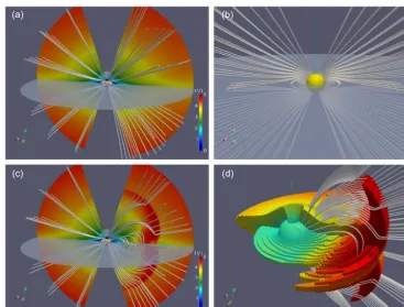
Figure 1.Perspective rendering of our model’s magnetic field and flow configuration.(a)Selected magnetic field lines (white) and absolute velocity in the poloidal planey=0 att=20, i.e., immediately prior to CME outbreak, showing a quiet Sun situation. The semitransparent disk marks the ecliptic plane.(b)Magnified view of the streamer belt of closed field lines (also att=20) emanating from the Sun’s surface (yellow sphere) shown using a different set of lines. The cusps of the outermost field lines extend to about 8.5R.(c)Same situation as above at a later timet=28, at which the CME has caused a considerable disturbance and restructuring of magnetic topology.(d)Two isocontours ofr2ρusing the same color coding forVras above, again amended with selected field lines. Note the CME’s shell-like spatial structure with its distinct ecliptic groove.
warrants magnetic solenoidality using a constrained trans-port method, thus eliminating the need for the previously em-ployed projection scheme. For more details on the code, see Kissmann et al. (2008) and Wiengarten et al. (2015).
Rather than using the full energy equation, we simply assume that pressure P and number density n are related via an isothermal equation of state P =c2nmp (mp denot-ing the proton rest mass) with an isothermal sound speed c=180 km s−1that corresponds to a plasma temperature of about 2.0 MK. This seems appropriate, given that we intend to compare our findings to the much simpler case of a con-stant radial flow and a magnetic field given analytically as a Parker spiral (Czechowski and Mann, 2010). Our equidistant numerical grid of size (Nr, Nθ, Nφ)=(290,72,180) cov-ers the spherical domain r∈ [1,30]R= [0.005,0.14]AU, θ∈ [0.1π,0.9π], andφ∈ [0,2π], implying a cell extension of1r=0.1Rin the radial direction and 2◦in both azimuth
and colatitude. The region within angular distanceθ0=0.1π from the polar axis (with its cell sizes tending to zero in theφ direction) is deliberately excluded to save computation time. This can be justified for a CME that is launched in the
equato-rial plane and is unlikely to cause noticeable distortions near the solar axis.
The fluid variables are initialized att=0 as a radially ex-panding flow:
n|t=0=n0(r/R)−3, (1)
V|t=0=er
(r/rc)c : r <2rc
2c : r≥2rc, (2)
with a base number densityn0=1014m−3and the critical (sonic) radius rc=GM/(2c2), at which Vr=c. The
ve-locity profile of Eq. (2) is chosen to be close to the clas-sical solar wind solution of Parker (1958) in order to war-rant sufficiently fast convergence into a stationary state and also to conserve radial mass flux (∼r2nVr) within r≤rc. The dipolar magnetic field used by Kleimann et al. (2009) had to be modified in its θ component in order to accom-modate mirror boundary conditions at bothθmin=θ0=0.1π andθmax=π−θ0=0.9π, and it now reads
B|t=0=
2 cosθ r3
er+
sinθ r3
" 1−
sinθ 0 sinθ
2#
in units of 4c√µ0n0mp≈83 µT. A derivation of Eq. (3) is provided in Appendix A.
Within the inner radial boundary layer, quantities n,Br, Bθ, andVθ=0 are kept fixed at their initial values. We en-force Vφ=rsinθ (with=2.7 µHz being the Sun’s
angular rotation frequency) and extrapolate Vr linearly in-wards without fixing a specific boundary value (except that no backflow into the Sun is permitted). Finally, Bφis fixed by keeping the field lines straight across the boundary, i.e., the quantity (rBr/Bφ)constant along any radial direction. The respective boundary conditions atrmaxandφmin,maxare outflowing and periodic.
This system is then self-consistently evolved until a suf-ficiently stationary state is reached at t=t1=24 (in units of the sound crossing timets=R/c≈1.5 h). This
station-ary state is characterized by a helmet-streamer-like belt of closed magnetic lines at the equator and open, almost radial field lines at higher latitudes. Along these open field lines, the plasma flow forms a Parker-like wind, while a static region (“dead zone”) forms under the closed equatorial field lines. The overall situation is thus reminiscent of a quiet solar min-imum configuration.
2.2 Modeling a CME eruption
CMEs are complex dynamical structures that come in a wide variety of morphologies and exhibit an equally wide range of physical parameters. Despite the wealth of observational data that have been accumulated and the modeling effort invested by the space-weather community, key questions about their origin and the physical mechanisms that govern their erup-tion and propagaerup-tion remain unanswered to this day. Details on CME modeling may be found in reviews by Jacobs and Poedts (2011) and Kleimann (2012) and the references given therein, while observational aspects have been summarized by, e.g., Webb and Howard (2012) and Howard (2015).
In the present context, our aim is merely to obtain a first assessment of how influential the passage of a CME can be on a nanodust population near the Sun and an indication of the type and expected magnitude of its effects. This justifies the use of a rather simple density-driven CME model (see, e.g., Groth et al., 2000), in which the CME is launched at the solar surface by a transient increase in the boundary value forn(but not forV) in the same manner and using the same parameters as already employed by Kleimann et al. (2009), except that the elaborate averaging method that was used by these authors to implement spherical solar boundary condi-tions on a Cartesian grid is no longer necessary in the present case. Note in particular that this model CME has no internal magnetic flux rope whatsoever but owes its magnetic struc-ture entirely to that of the helmet streamer, which it is able to open up and push outwards by virtue of its increased gas pressure. The mass of the CME as described by the model is about 5.7×10¹³kg, which puts the CME in the moderate to strong class.
[image:4.612.308.548.66.238.2]-1
Figure 2.Plasma radial velocity profiles in the model along the directionθ=67◦,φ=189◦at the initial time of the CME (t=24) and 0.25 days later (t=28).
The CME departs from a circular patch of radius 30◦ cen-tered on theθ=π/2,φ=0 direction, causing a temporary rupture of field line connectivity as it expands and travels out-wards, reaching peak speeds of about 5c≈900 km s−1. The simulation is halted attend,MHD=t2=50, at which time the CME has completely left the computational volume, which has again returned to a quiescent state. The numerical data for the entire CME expansion process thus cover a time pe-riod of 26tc∼1.6 days.
The respective MHD configurations of the quiet Sun and during CME passage are illustrated in the panels of Fig. 1, and velocity profiles for both instants are shown in Fig. 2.
For numerical convenience, the plasma configuration {V,B}is then interpolated linearly both on the spatial grid and between consecutive time frames of separation1t=1.
3 Particle simulations
Our calculations are similar to those in Czechowski and Mann (2010, 2012) but with the simple time-stationary an-alytical model of the solar wind replaced by the time-dependent numerical MHD solution corresponding to the model CME.
The electric charge of nanodust cannot be reliably esti-mated, so we have to use an extrapolation from the results for the larger grains (Mukai, 1981; Kimura and Mann, 1998). In the calculations we use two sample values of the charge-to-mass ratio:Q/m=10−4e/mp(for the grain radiuss∼3 nm with ∼8 V surface potential) and Q/m=10−5e/mp (for s∼10 nm with∼9 V surface potential).
the frequency of Larmor rotation (Czechowski and Mann, 2010, 2012). As a result, the particle motion can be approx-imated by replacing the fluctuating electric charge with the time-averaged value. We assume that this average is approx-imately constant within the computational domain.
The equation of motion for a nanodust particle with mass m, electric chargeQ, and velocityvbecomes
dv
dt = Q
mc(v−V)×B−
GM
r2 er+Fγ+Fion, (4) where v=dr/dt is the particle velocity and r the particle position. The first term on the right-hand side of Eq. (4) in-cludes the electric field E= −(1/c)V×B induced by the solar wind plasma flow, which is responsible for a large part of acceleration that a charged particle experiences in the sim-ulation.
Fγ=
GM
r2 β h
1−vr c
er− v
c i
(5) is the force due to solar radiation, the Poynting–Robertson force (Robertson, 1937). Since the radiation pressure-to-gravity ratioβfor nanodust is expected to be small (β∼0.1), in most of the calculations presented here we setβ=0, ne-glecting the Poynting–Robertson force.
In some calculations we also includedFion, the drag force caused by solar wind proton impacts on a grain:
Fion= −FSW(r)CSW,p
v−V
|v−V|, (6)
whereFSW(r)=nSW(r)mp|v−V|2is the solar wind proton flux at r relative to the dust grain, andCSW,p is given by Minato et al. (2004):
CSW,p=π a2 2 3
2a
l(E)(2a≤l(E)), (7)
CSW,p=π a2 "
1−1 3
l(E) 2a
2#
(2a > l(E)). (8)
Here, a is the radius of the grain, and l(E) is the range of a proton of initial energy E=(1/2)mp|v−V|2 passing through the material of the grain. Following Minato et al. (2004) we assumel(E)∝E1/2withl(1 keV)=0.092 µm for silicate grains. Similarly to Minato et al. (2004), we simplify the proton drag force by neglecting the thermal component of the proton velocity. The drag force is weak compared to other forces. For the MHD solution used in our simulations, its magnitude along a sample of nanodust trajectories varies between∼2 and∼10 % of the gravity force with approxi-mately the same range for the CME and the time-stationary configurations.
Equation (4) is solved numerically by the Runge–Kutta method with linear interpolation used to incorporate the re-sults (V andB) from the MHD simulation.
The initial conditions forr andv are defined as follows. We assume that the nanodust particles are released at zero
D
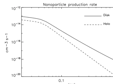
[image:5.612.314.539.63.230.2]H
Figure 3.Nanodust creation rate as a function of the heliocen-tric distance assumed in our calculations (Czechowski and Mann, 2010).
relative velocity from the parent bodies in circular Keple-rian orbits. The orbits are specified by the radiusr, the di-rection of the ascending nodeψ, and the inclinationδ. As in Czechowski and Mann (2010), we disregard the difference between the solar equator and the ecliptic plane so that the inclinationδis defined relative to the solar equatorial plane. The initial position of the particle on the orbit is specified by the azimuthal angleα. We choose nr=10 values of r (0.01 AU< r <0.135 AU, logarithmic spacing),nψ=4 val-ues ofψ(22.5◦< ψ <157.5◦),nδ=12 values ofδ(−66◦< δ <66◦), and nα=10 values of α (18◦< ψ <342◦). One sample therefore consists of 4800 trajectories.
Most of our particle simulations stay within the time limits of the MHD model for the CME (time fromt1=24 tot2 = 50, total time length∼1.6 days). We also use time-extended plasma configurations, which consist of the CME solution in the (t1,t2) time interval and the time-stationary configuration outside. We assume that the time-stationary configuration for t < t1can be approximated by thet=t1=24 time frame and fort > t2by thet=t2=50 time frame of the original MHD solution.
The initial and (maximum) final times for particle motion are taken to be the same for all particles in the sample. All simulations presented here (also including the time-extended calculations) start from the same initial time equal tot1+1t, where1t=2.6 in dimensionless MHD time units (∼0.16 days). The particle simulations restricted to the model CME end att2−1t so that the time length of each of them is ∼1.32 days.
To calculate the averages over the ensemble of the initial conditions, we have to assign probability weights to the ini-tial points. For any quantity A(r)dependent on the initial pointr, we define the averagehAias
hAi = R
d3rn(r)A(r) R
wheren(r)is the nanodust creation rate at the pointr, and the integration runs over the region over which the initial points are distributed. We want to approximate the volume integral by the weighted sum over the set of our initial points. In spherical coordinates (heliocentric distance r, heliographic colatitude θ, and heliographic longitude φ), the region of space containing the initial points (0.02 AU≤r≤0.12 AU, 18◦≤θ≤162◦, 0◦≤φ≤360◦) is divided into 800 bins cen-tered at the pointsri (i=1 to 10),θj (j=1 to 10), andφk (k=1 to 8) with equal spacings between logri,θjandφk. An initial pointrI(I =1 to 4800), which belongs to the(i, j, k) bin, is assigned a weightwI equal to the volume of the bin multiplied byn(ri)/N, wheren(r)is the assumed nanodust creation rate at the heliocentric distance r (see Fig. 3) and N is the number of initial points belonging to the bin. If the initial point corresponds to the orbit with low inclination (|δ| ≤13.5◦), thenn(r)=nd(r)(the rate for the dust disk); otherwisen(r)=nh(r)(the rate for the dust halo). The aver-agehAiis then approximately given by
hAi ≈ P
wIA(rI) P
wI , (10)
where the sum over all initial points isrI.
For comparison, we also repeated the calculations with a different approximate expression for the sum over the initial states used by Czechowski and Mann (2010). The results for escape rates were higher by a factor of∼1.3, but our quali-tative conclusions were not affected.
We use the same nanodust creation rates as Czechowski and Mann (2010). The nanodust creation rates inside the circumsolar dust disk (nd(r)) and in the dust halo around the Sun (nh(r)) are shown in Fig. 3. These rates were found to underestimate the nanodust flux derived by STEREO/WAVES (Czechowski and Mann, 2011b; Mann and Czechowski, 2012). However, as can be seen from Eq. (10), our results do not depend on the absolute values of the nanodust production rates.
The dust–dust collision and fragmentation model used for calculating the rates is described in Mann and Czechowski (2005) and based on Grün (1985). The mass distributions of dust in the circumsolar cloud are modified versions (Mann and Czechowski, 2005) of the interplanetary flux model by Grün (1985). The spatial distributions are proportional to ∼r−1in the disk andr−2in the halo regions, both flatten-ing forr <10R. The velocities of collisions between the
dust grains (the parent bodies of the nanodust) are assumed to scale asr−1/2.
4 Results
We present the results of simulations for different cases listed in Table 1. The computational domain in space is limited to the region described by the CME solution (see Sect. 2). In each simulation, we follow the motion of a sample of
4800 particles. The distribution over the initial points is the same for all cases. In each sample, the initial time, the values of the charge-to-mass ratioQ/m, and the radiation pressure-to-gravity ratioβ are the same for all particles. The distri-butions shown in the figures (Figs. 4, 5, 6, 7, 10, and 16) are obtained after weighing the results with the assumed nanoparticle production rate (Fig. 3), as described in Sect. 3, Eq. (10). The distributions over final values mean the dis-tributions over values reached by particles at the end of the calculations (the moment of escape or reaching the final time limit). The bins have equal size. The plotted fractions sum to 1 when the non-escaping (solid lines) and escaping (dashed or dotted lines) populations are combined.
In Table 1, “CME” denotes the calculation using the orig-inal MHD solution for the CME (total time span 1.6 days), “CME+stationary” is the time-extended configuration (the CME followed by the final time frame of the CME), and “sta-tionary” means that the final frame of the CME was used as a time-independent distribution for the whole time period. The “time length” column lists the differences between the final and initial times used in particle calculations. These are taken a little shorter than the total time length of the cor-responding background plasma configuration. The “(1−β)” notation means that the gravity force in the equation of mo-tion (Eq. 4) is multiplied by (1−β) withβ=0.1. “PR” means that the full Poynting–Robertson force (Eq. 5) withβ=0.1 is included. Apart from these two cases, the value ofβ was set to zero. “Drag” denotes the results including the effect of the plasma ion drag force (Eq. 6). “Trapped” means that only the trajectories in the trapped class (see Sect. 5.3) are included, and fesc denotes the (weighted) fractions of the escaping particles (rapid or slow) calculated using Eq. (10). The (unweighted) numbers of escaping trajectories are given in brackets below the correspondingfesc. The total number of trajectories is 4800 for each case, except the last two. The non-escaping fraction for each case is equal to 1 minus the sum offescvalues for rapid and slow populations.
4.1 Rapidly escaping population
A significant fraction of particles (Table 1) escapes from the computational domain within the time extent (1.6 days) of the original CME solution. Particles escape predominantly across the outer boundary (r=0.14 AU) of the computa-tional domain. Only a small fraction (∼1.5 %, ∼200 tra-jectories) crosses the inner boundary (r=0.005 AU), and an even smaller fraction (∼0.7 %,∼10 trajectories) crosses the boundary in solar colatitude (θ=18◦or 162◦). Inclusion of the ion drag force increases the fraction of particles escaping through the inner boundary (∼3 % ,∼650 trajectories within 1.6 days).
Table 1.Escape fractionsfescfor rapidly and slowly escaping populations.
No. Q/m Time length Case fesc fesc
(e/mp) (days) (rapid) (slow)
(1) 10−5 1.32 CME 0.37
(1567)
(2) −10−5 1.32 CME 0.34
(1441)
(3) 10−5 1.32 Stationary 0.003
(72)
(4) −10−5 1.32 Stationary 0.004
(106)
(5) 10−5 2.99 CME+stationary 0.37 0.13
(1563) (575)
(6) 10−4 1.32 CME 0.33
(1683)
(7) 10−5 1.32 CME, (1-β) 0.38
(1555)
(8) 10−5 1.32 CME, drag 0.39
(1977)
(9) 10−5 6.11 CME+stationary 0.37 0.21
(1563) (1176)
(10) 10−5 6.11 CME+stationary, PR 0.38 0.22
(1551) (1256)
(11) 10−5 6.11 CME+stationary, drag 0.39 0.29
(1551) (1256)
(12) 10−5 6.11 Stationary 0.002 0.36
(72) (1364)
(13) 10−5 76.4 CME+stationary, trapped 0.30
(1829 trajectories) (959)
(14) 10−5 33.0 CME+stationary, drag 0.79
(1094 trajectories) (864)
qualitatively similar. Taking into account the effect of the ra-diation pressure (the(1−β)factor in the gravity force or the full Poynting–Robertson force term) does not greatly affect the results (Fig. 5b) because of the small value ofβ (∼0.1) used for the nanodust particles. The effect of the ion drag force on the velocity distribution of rapidly escaping particles is also small. The∼2 % increase in the escaping fraction (Ta-ble 1) is due to particles escaping through the inner boundary. If the CME is replaced by the time-stationary model, the es-caping particles are essentially absent (Fig. 5c).
In heliographic longitude φ, the region of origin for the majority of the rapidly escaping particles lies between 75 and 285◦ (Fig. 6), which coincides with the region where the plasma flow and magnetic field perturbations associated
with the CME were the strongest. The non-escaping particles originate mostly outside of this region.
-1
F
N
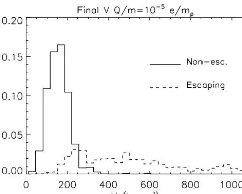
[image:8.612.310.548.30.596.2]E
Figure 4.Distribution of the final velocity for non-escaping and es-caping particle populations obtained in the CME model for a sample of 4800 nanodust particles withQ/m=10−5e/mp.
plasma flow. The final velocity is within a factor of 2 from that of the local plasma. The magnetic field lines have the form of expanding arcs (Fig. 8) or, very close to the solar equator, of magnetic islands carried outwards with the flow (Fig. 9). In the latter case, the trajectories often show mul-tiple crossings of the solar equator plane at z=0 (Fig. 9). This occurs for the negative grain charge, for which the field polarity is “focusing”, but also for the positive charge (“de-focusing” polarity). Note that the peak in finalθ (Fig. 7) is less prominent for the focusing configuration.
4.2 Particles escaping after the end of the CME: the slowly escaping population
The loss of particles from the computational domain con-tinues after the end of the CME. The final velocity distri-bution obtained for the time-extended model (CME+the time-stationary period, total time length ∼6 days, Fig. 10) includes three components: non-escaping particles (solid lines), particles escaping during the CME (rapidly escap-ing particles, dashed lines), and the particles escapescap-ing after the end of the CME (slowly escaping particles, dotted lines). The slowly escaping particles have a narrow velocity distri-bution (Fig. 10a) strongly suppressed beyond∼250 km s−1. Acceleration of nanodust particles to very high velocities (∼1000 km s−1) is therefore restricted solely to the CME time period.
The distribution of the initial heliographic longitudeφfor slowly escaping particles (Fig. 10c) is similar to that for non-escaping particles. Unlike the rapidly non-escaping particles, the slowly escaping particles (Fig. 10b) have no sharp central peak in the distribution of finalθvalues.
-1
F
N
E
F
N E
F
N
E
-1
-1
Figure 5. As Fig. 4 but for the following cases: (a) Q/m=
10−4e/mp, (b) Q/m=10−5e/mp with gravity modified by the factor(1−β), β=0.1, and(c)Q/m=10−5e/mp for the time-stationary plasma configuration (initial time frame of the CME so-lution).
[image:8.612.48.287.65.257.2]N
[image:9.612.47.288.66.258.2]E
Figure 6.As Fig. 4 but for the distribution in initial heliographic longitude.
by the particles escaping through the lower (rmin) boundary. The final velocity distribution of slowly escaping particles (Fig. 11) differs from that for the no-drag case by having a second peak at∼300 km s−1, representing particles escaping across the lower boundary. The distributions in final θ and initialφare similar to those of the no-drag case.
Figure 13 shows the fractions of nanodust surviving from the sample of particles created at the same initial moment as a function of time for the cases with and without ion drag. For the particles escaping between the end of the CME and the end of the period covered by the calculations, the exponen-tial fit of the form(A−B)exp(−t /τ )+Bgivesτ≈1.9 days andB=0.37 (without drag) andτ ≈2.9 days andB=0.19 (with drag). If the behavior of the surviving particle fraction were described by the exponential formula, the value of B would be equal to the asymptotic value of the surviving frac-tion.
We performed additional time-extended simulations to es-timate the surviving particle fraction after a longer time pe-riod. The results were the following: with drag included, 6 % survived after 33 days (Fig. 12); without drag, 25 % survived after 76 days. In the latter case, only trapped particles were included in the simulation.
4.3 Trapped particles
4.3.1 Trapping and the guiding center approximation Although the guiding center approximation is not used in our simulations, it was found to be helpful in understand-ing the trappunderstand-ing mechanism of nanodust in the vicinity of the Sun (Czechowski and Mann, 2010, 2012). In this section we briefly summarize the argument leading to the phase space model of Czechowski and Mann (2010, 2012).
F
E
N
[image:9.612.306.548.67.474.2]E
N
F
Figure 7.The distributions over final values of solar colatitudeθfor the nanodust particles with(a)Q/m=10−5e/mpand(b)Q/m=
−10−5e/mp. For escaping particles (dashed line), there is a narrow peak near the solar equator (θ=π/2) for both signs ofQ.
The equations for the parallel componentv||Gand the per-pendicular partvGT of the velocity of the guiding center are (Northrop, 1958)
dv||G
dt =g||−µ∂SB+VT ·∂t ˆ b
+VT·
(VT · ∇)bˆ+v||G∂Sbˆ
, (11)
vGT =VT, (12)
wherebˆ=B/B, g|| is the component of the gravity force
-1
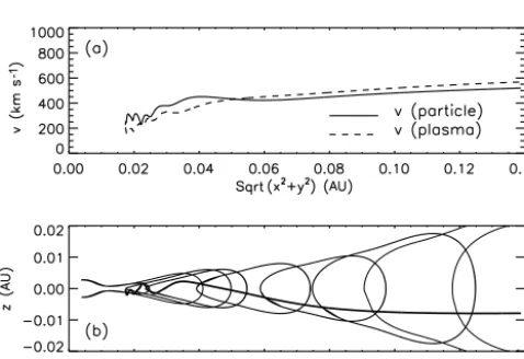
S
S
Figure 8. (a)The particle and plasma speed and(b)the magnetic field structure along the trajectory of a rapidly escaping particle withQ/m=10−5e/mp. The thin lines in panel(b)are the selected magnetic field lines encountered by the particle along its trajectory, which is shown as the thick line. The coordinatezis measured along the solar rotation axis withz=0 at the solar equator.
-1
S
[image:10.612.50.289.64.230.2]S
Figure 9.As Fig. 8 but the selected particle has a negative charge (Q/m= −10−5e/mp) and is released closer to the Sun.
invariant, andv0
T = |vT −VT|is the perpendicular speed of the particle in the plasma frame. In Eq. (12) the non-leading Q/m-dependent drift terms are omitted. With this additional approximation, the particle (the guiding center) slides along the magnetic field line convected with the plasma flow.
In the study by Czechowski and Mann (2010, 2012) it is assumed that the plasma flow and the magnetic field are time stationary with the plasma flow purely radial and the mag-netic field in the form of the Parker spiral:
ˆ
b= er−aeφ
(1+a2)1/2 B= C r2(1+a
2)1/2, (13) wherea=(r/V )sinθ,is the angular velocity of solar
rotation,V is the solar wind speed, andθis the heliographic colatitude.C is constant along a magnetic field line and can
F
N
R
S
F
N
R
S
-1
N
R
S
Figure 10.Distributions of(a)final velocity, (b)final colatitude, and(c)initial longitude for the time-extended case (CME followed by the time-stationary configuration) lasting∼6 days. The distri-butions for non-escaping, rapidly escaping (escaping during the CME), and slowly escaping particles (escaping after the end of the CME) are shown.
[image:10.612.310.550.65.606.2] [image:10.612.49.288.320.484.2]-1
F
N
R
[image:11.612.308.549.64.259.2]S
Figure 11.As Fig. 10a but for the simulation including the plasma ion drag.
[image:11.612.47.289.65.237.2]T
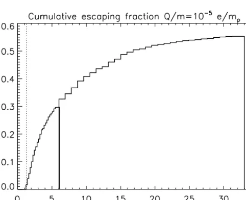
Figure 12.Cumulative fraction of particles escaping from the com-putational domain as a function of time for a time-extended (33 days long) simulation including the ion drag. Rapidly escaping particles (39 %) are not included in the figure. The result implies that only
∼6 % of all particles remain inside at the end of the calculation: 100–39 % (rapidly escaping),−55 % (present figure). A rough esti-mation of the characteristic escape time gives∼10 days.
The sliding motion is determined by the force terms in Eq. (11), which can be explicitly calculated using Eq. (13). We restrict attention to thea1 region (corresponding to r1 AU). There is an inward-directed gravity force g||= −
GM(1−β)
r2 , (14)
including the correction β due to radiation pressure. The outward-directed forces are the “magnetic mirror” force −µ∂SB= |v0T0|
2r2 0/r
3 (15)
S
R
E
N
D
T
Figure 13.The fraction of particles remaining inside the calculation region as a function of time for the CME time-extended models with and without the ion drag. The vertical dotted line marks the end of the CME. The dashed lines shows the two parameter (Bandτ) fits of the form(A−B)exp(−t /τ )+Bapplied for the time period starting 1.32 days after the initial time. The best fits giveB=0.37 andτ=1.87 days without drag andB=0.19,τ=2.9 days with drag.
and the “centrifugal” force
VT ·(VT · ∇)bˆ=2rsin2θ. (16)
Here,v0
T0 is the initial transverse velocity of the nanodust particle in the plasma frame at the heliocentric distancer0, where the particle is released from the parent body. The trap-ping occurs if the gravity force stops the particle outward motion before the “centrifugal” force becomes dominant.
A more detailed analysis (Czechowski and Mann, 2010, 2011a, 2012) shows that, in the region where a1, the guiding center motion is described by the equations
dr/dt=v, (17)
dv/dt=W (r)−(a2/r)v2, (18)
whereris the heliocentric distance of the guiding center,v is the radial component of the guiding center velocity, and
W (r)=GM(1−β) r2
" −1+r2
r + r
r1 3#
[image:11.612.48.289.285.481.2]T
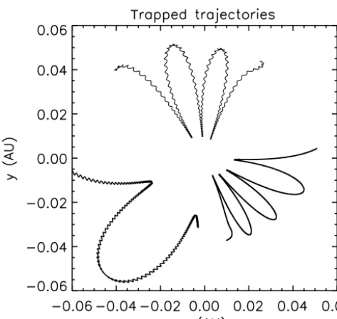
Figure 14.Trapped particle trajectories projected onto the (x,y) plane. The top (Q/m=10−5e/mp) and bottom right (Q/m=
10−4e/mp) trajectories follow from simulations for the case of the time-extended (6.11 days long) CME model. For comparison, a tra-jectory obtained in the model with constant plasma speed and Parker spiral magnetic field is shown in the lower left part of the figure.
Here, r2=
|v0T0|2r02 GM(1−β)
, (20)
r1=
GM(1−β) 2sin2θ
!1/3
. (21)
Note that the gravity force (Eq. 14) forr > r2dominates over the magnetic mirror force (Eq. 15) and forr < r1 over the centrifugal force (Eq. 16).
Equations (17) and (18) define the dynamical system in the (r, v)phase plane. IfW (r)=0 has real roots, the fixed points appear at the root positions on theraxis in the(r, v)plane. Ifr2r1, the fixed points are approximately atr≈r2and r≈r1. The trapped orbits encircle the fixed pointr≈r2. The fixed pointr≈r1is the outer boundary of the trapped region. In the solar system, r1≈(0.16AU )(1−β)1/3sin−2/3θ. Since the CME model is limited tor <0.14 AU, all our sim-ulations are restricted to ther < r1region.
4.3.2 Trapped particles: simulation results
As explained in the previous subsection, the motion of a trapped particle in the simple time-stationary model (Czechowski and Mann, 2010, 2012) consists of sliding be-tween the two turning points along a rotating magnetic field line. A class of particles with similar trajectories was identi-fied in our results. Two examples, projected onto the(x, y)
T
R
S S
T
R
T T
T T
[image:12.612.309.539.73.531.2]T T
Figure 15.Distance versus time plots for a sample of trajecto-ries of the nanodust particles (Q/m=10−5e/mp) belonging to(a) “rapidly escaping”,(b)“slowly escaping”, and(c)“trapped” popu-lations.
Figure 16.Distribution of the difference1φbetween the final and initial values of the heliographic longitudeφfor the particles in the “trapped” class for the case of the time-extended (6.11 days long) CME model. The vertical dotted line shows the value of1φ corre-sponding to solar rotation over 6.11 days.
N
D
Figure 17. Effect of the (photon) Poynting–Robertson force and the plasma drag force on a trapped particle trajectory. While the Poynting–Robertson force leaves the minimum and maximumr val-ues almost unaffected, the plasma drag causes them to decrease with time. The decrease in minimumrmay lead to crossing of the lower boundary of the calculational domain and/or destruction of the nan-odust particle by sublimation.
We required that the oscillations in r persist for the whole time span of the trajectory and that at least one full cycle of radial oscillation (e.g., a particle starting from the upper turning point must return to it at least once) is present.
Figure 16 shows the distribution of the gain1φin the he-liographic longitude (the difference between the final and initial values of φ) achieved after 6.11 days by the
parti-cles in the trapped class. Although some spread can be seen, there is a sharp maximum in the distribution close to the an-gle (86.6◦) corresponding to the angle of Carrington rotation
over the period of 6.11 days. This is consistent with trapped particles staying close to a rotating magnetic field line, as suggested by the guiding center approximation.
The particles in the trapped class constitute the majority of particles that remain inside the computational domain af-ter the extended period of∼6 days starting with the CME. Since the orbits of particles in the trapped class evolve with time, some of these particles may ultimately escape from the calculational volume. We attempted to estimate the charac-teristic time for escape of trapped particles in the absence of plasma ion drag force by extending the simulation time to about 76 days from the beginning of the CME. We found the majority (70 %) of trapped particles remaining inside the region.
Assuming that the nanodust particles are created continu-ously, the trapped nanodust would accumulate in the vicin-ity of the Sun until some loss mechanism balanced the cre-ation rate. Our calculcre-ations suggest that the main loss mech-anism may be due to the plasma ion drag. The ion drag force causes contraction of the orbits of trapped particles (Fig. 17), leading to a decrease in the aphelium and the perihelium dis-tances and, in many cases, to the particle crossing the inner boundary and falling into the Sun. This process is responsible for the∼11 % increase in the slowly escaping particle frac-tion noted in the previous subsecfrac-tion. The contracfrac-tion rate of trapped orbits depends on their initial parameters and occurs particularly fast for particles created near the lower bound-ary.
The result of the long-term (33 days) simulation (Fig. 12) including the effect of drag permitted us to roughly estimate the average characteristic escape time for nanodust (exclud-ing the rapidly escap(exclud-ing population) to be on the order of 10 days.
4.4 Loss through sublimation
The lifetime of small dust grains in the vicinity of the Sun, particularly those belonging to the trapped class, can be lim-ited by sublimation and sputtering. An estimation (ignoring the effect of the ion drag) was made by Czechowski and Mann (2010) based on the results of Krivov et al. (1998) for sublimation and Mukai and Schwehm (1981) for sputtering. The survival probability against sputtering after 100 orbits for 10 nm particles released from low-inclination orbit was found to be 0.5 for the initial heliocentric distance 0.12 AU, increasing to 0.8 for the initial distance within 0.06 AU from the Sun.
[image:13.612.48.289.344.527.2]dis-tance of 3Rwith the sublimation time for a 100 nm particle
equal to 0.01 years. Assuming that the lifetime of a spheri-cal sublimating particle is proportional to its radius, for the particular case of the time-extended (6.11 days long) sim-ulation (including the ion drag force) forQ/m=10−5e/mp particles with the radius 10 nm, we obtain the loss fraction by sublimation after∼6 days to be 15 % with 14 % contributed by particles in the trapped class. The result without the ion drag force would be 4.5 % with 4.1 % due to trapped parti-cles.
5 Conclusions
We present the results of numerical simulations of the mo-tion of nanodust particles released from circular Keplerian orbits between 0.005 and 0.14 AU from the Sun with the so-lar wind flow and the magnetic field approximately corre-sponding to the MHD model of the CME by Kleimann et al. (2009). The mass of the CME as described by the model is about 5.7×10¹³kg, which puts the CME in the moderate to strong class. The MHD model includes a simplifying as-sumption that the solar equator is the same as the solar mag-netic equator.
In part of our calculations we include the plasma ion drag force, which was omitted in the earlier work on nanodust dy-namics near the Sun (Czechowski and Mann, 2010, 2012). We follow the approach of Minato et al. (2004). We find that the ion drag force plays a very important role in nanodust dynamics.
In a simple time-stationary model of the solar wind with constant radially directed velocity and the Parker spi-ral form of the magnetic field, the nanodust released from low-inclination circular orbits within the regionr <0.14 AU would be trapped (Czechowski and Mann, 2010, 2012). Al-though the MHD solution used in the present study is very different from this simple model, we find that a similar trap-ping mechanism operates for a significant fraction (∼35 %) of nanodust particles.
About 35 % of the nanodust particles released during the CME form the rapidly escaping population with a broad ve-locity distribution extending to 1000 km s−1. These particles come from the region where the disturbance of plasma flow and magnetic field caused by the CME is strong. The accel-eration process is associated with the regions of closed mag-netic field lines: the expanding arcs in the CME region and the narrow belt in the vicinity of the solar equator plane.
The remaining particles, which belong to neither the rapidly escaping nor the trapped class, escape from the region after the time span (∼1.6 days) of the model CME. These particles form the slowly escaping population. To investigate their behavior, we extended the calculations beyond the time span of the CME, assuming that the CME is followed by a pe-riod described by a time-stationary MHD solution. We found that the ion drag force becomes important for time-extended simulations.
The ion drag force differs from other forces (Lorentz, grav-ity, and Poynting–Robertson) included in our calculations by its destructive effect on trapped particle trajectories. The trapped orbits contract and ultimately cross the inner bound-ary. The lifetime of trapped particles is consequently limited by the ion drag force. From our simulations, we estimated the average lifetime of nanodust to be∼10 days.
The effect of the ion drag on particle trajectories increases the nanodust destruction rate due to sublimation. Assum-ing that the results of Krivov et al. (1998) can be applied to nanodust, we estimated the fraction of nanodust parti-cles destroyed by sublimation over the period of∼6 days (1.6 days CME+time-stationary period) to be 15 % com-pared to 4.5 % if the ion drag is neglected. Almost all nanodust particles destroyed by sublimation belong to the trapped population.
Since our computational domain was restricted to r < 0.14 AU, we cannot directly compare our results with the ob-servations by STEREO/WAVES in the vicinity of the Earth’s orbit, as discussed by Le Chat et al. (2015). To estimate the flux of charged nanodust away from the source, it is neces-sary to have a reliable model of nanodust propagation to the observation point (see Juhasz and Horanyi, 2013). For com-parison with the observations, the simulations would have to be extended to cover a wider region of space up to∼1 AU from the Sun. Also, the model of the CME would have to be modified to include the more realistic situation of the solar magnetic equator inclined relative to the solar equator plane.
Appendix A: Fixing the initial magnetic field The usual magnetic field of a point dipole, which reads
B=
2 cosθ r3 ,
sinθ r3 ,0
(A1) in spherical coordinates(r, θ, ϕ), derives from a vector po-tentialA=(sinθ/r2)eϕ via
Br, Bθ, Bϕ = B= ∇ ×A (A2)
= 1
rsinθ ∂
∂θ sinθ Aϕ
,−1 r
∂ ∂r r Aϕ
,0
and has radial field lines only atθ∈ {0, π}. We now wish to modify this field such that the field lines become radial at a colatitudeθ0that may be freely specified, while maintaining the same magnetic flux through the surfacer=R. For this
purpose, we first note from Eq. (A2) that the transformation
sinθ Aϕ →sinθ Aϕ,mod+f (r) (A3)
leavesBr unchanged for any functionf (r). This gauge free-dom in the choice off (r)may be exploited to haveBθvanish atθ=θ0:
0=! Bθ|θ0 = − 1 r ∂ ∂r r Aϕ+
f (r) sinθ θ 0
= −1 r ∂ ∂r sinθ 0 r +
r f (r) sinθ0
, (A4)
from which we get sinθ0
r +
r f (r) sinθ0
=C⇒f (r)=
C−sinθ0 r
sinθ 0
r (A5)
withCa constant of integration. The resultingBθcomponent becomes
Bθ,mod = − 1 r ∂ ∂r r sinθ r2 +
1 sinθ
C−sinθ0 r sinθ 0 r = 1 r3 "
sinθ−sin 2θ
0 sinθ
# =Bθ
" 1−sin
2θ 0 sin2θ
# . (A6)
SinceBθ,modis obviously independent ofC, we may choose C=0 and finally obtain
Amod =
sinθ r2 " 1− sinθ 0 sinθ 2#
eϕ (A7)
Bmod =
2 cosθ r3
er+
sinθ r3 " 1− sinθ 0 sinθ 2#
eθ (A8)
Author contributions. AC performed the nanodust simulations and analysis of the results. JK designed the MHD model of the CME.
Competing interests. The authors declare that they have no conflict of interest.
Acknowledgements. We thank the referee for the important sugges-tion to include the ion drag term in our calculasugges-tions. We are grateful to Horst Fichtner for helpful comments, discussions, and support, as well as to Ralf Kissmann for valuable technical assistance with his CRONOS code. Furthermore, Jens Kleimann acknowledges fi-nancial support from the Deutsche Forschungsgemeinschaft (DFG) via grant FI 706/8-2 and from the Ruhr Astroparticle and Plasma Physics (RAPP) Center, funded as MERCUR grant St-2014-040.
The topical editor, Elias Roussos, thanks two anonymous refer-ees for help in evaluating this paper.
References
Czechowski, A. and Mann, I.: Formation and Acceleration of nano Dust in the Inner Heliosphere, Astrophys. J., 714, 89–99, 2010. Czechowski, A. and Mann, I.: Formation and Acceleration of nano
Dust in the Inner Heliosphere: Erratum, Astrophys. J., 732, p. 127, 2011a.
Czechowski, A. and Mann, I.: Formation and Acceleration of nano Dust in the Inner Heliosphere: Erratum, Astrophys. J., 740, p. 50, 2011b.
Czechowski, A. and Mann, I.: Nanodust dynamics in the inter-planetary space, in: Nanodust in the Solar System: Discoveries and Interpretations, edited by: Mann, I., Meyer-Vernet, N., and Czechowski, A., Springer 2012, p. 47, 2012.
Groth, C. P. T., De Zeeuw, D. L., Gombosi, T. I., and Powell, K .G.: Global three-dimensional MHD simulation of a space weather event: CME formation, interplanetary propagation, and interac-tion with the magnetosphere, J. Geophys. Res., 105, 25053– 25078, 2000.
Grün, E., Zook, H. A., Fechtig, H., and Giese, R. H.: Collisional balance of the meteoritic complex, Icarus, 62, 244–272, 1985. Grün, E., Zook, H. A., Baguhl, M., Balogh, A., Bame, S.J., Fechtig,
H., Forsyth, R., Hanner, M.S., Horanyi, M., Kissel, J., Lindblad, B.-A., Linkert, D., Linkert, G., Mann, I., McDonnell, J.A.M., Morfill, G.E., Phillips, J.L., Polanskey, C., Schwehm, G., Sid-dique, N., Staubach, P., Svestka, J., and Taylor, A.: Discovery of jovian dust streams and interstellar grains by the Ulysses space-craft, Nature, 262, 428–430, 1993.
Howard, T. A.: Regarding the detectability and measurement of coronal mass ejections, J. Space Weather and Space Climate, 5, 15 pp., 2015
Ip, W.-H. and Yan, T.-H.: Injection and acceleration of charged nano-dust particles from sungrazing comets, in: Physics of the heliosphere: a 10 year retrospective, Proc. of the 10th Annual In-ternational Astrophysics Conference, AIP Conference Proceed-ings, 1436, 30–35, 2012.
Jacobs, C. and Poedts, S.: Models for coronal mass ejections, J. Atmos. Sol.-Terr. Phys., 73, 1148–1155, 2011.
Juhasz, A. and Horanyi, M.: Dynamics and distribution of nano-dust particles in the inner solar system, Geophys. Res. Lett., 40, 2500–2504, 2013.
Kimura, H. and Mann, I.: The electric charging of interstellar dust in the solar system and consequences for its dynamics, Astrophys. J., 499, 454–462, 1998.
Kissmann, R., Kleimann, J., Fichtner, H., and Grauer, R.: Local tur-bulence simulations for the multiphase ISM, Monthly Not. Royal Astron. Soc., 391, 1577–1588, 2008.
Kleimann, J., Kopp, A., Fichtner, H., and Grauer, R.: A novel code for numerical 3-D MHD studies of CME expansion, Ann. Geo-phys., 27, 989–1004, 2009.
Kleimann, J.: 4π models of CMEs and ICMEs (Invited Review), Sol. Phys., 281, 353–367, 2012.
Krivov, A. Kimura, H., and Mann, I.: Dynamics of Dust near the Sun, Icarus, 134, 311–327, 1998.
Le Chat, G., Zaslavsky, A., Meyer-Vernet, N., Issautier, K., Belheouane, S., Pantellini, F., Maksimovic, M., Zouganelis, I., Bale, S. D., and Kasper, J. C.: Interplanetary nan-odust detection by the Solar Terrestrial Relations Observa-tory/WAVES low frequency receiver, Sol. Phys., 286, 549–559, https://doi.org/10.1007/s11207-013-0268-x, 2013.
Le Chat, G., Issautier, K., Zaslavsky, A., Pantellini, F., Meyer-Vernet, N., Belheouane, S., and Maksimovic, M.: Effect of the Interplanetary Medium on Nanodust, Observations by the So-lar Terrestrial Relations Observatory, SoSo-lar Phys., 290, 933–942, https://doi.org/10.1007/s11207-015-0651-x, 2015.
Mann, I., Kimura, H., Biesecker, D. A., Tsurutani, B. T., Grün, E., McKibben, R. B., Liou, J. C., MacQueen, R. M., Mukai, T., Guhathakurta, M., and Lamy, P.: Dust near the Sun, Space Sci. Rev., 110, 269–305, 2004.
Mann, I. and Czechowski, A.: Dust Destruction and Ion Formation in the Inner Solar System, Astrophys. J. Lett., 621, L73–L76, 2005.
Mann, I., Murad, E., and Czechowski, A.: Nanoparticles in the inner solar system, Planet. Space. Sci., 55, 1000–1009, https://doi.org/10.1016/j.pss.2006/11.015, 2007.
Mann, I. and Czechowski, A.: Causes and consequences of the ex-istence of nanodust in interplanetary space, in: Nanodust in the Solar System: Discoveries and Interpretations, edited by: Mann, I., Meyer-Vernet, N., and Czechowski, A., Springer, 2012, 195– 219, https://doi.org/10.1007/978-3-642-27543-2, 2012. Mann, I., Meyer-Vernet, N., and Czechowski, A.: Dust
in the planetary system: dust interactions in space plasmas of the solar system, Phys. Rep., 536, 1–39, https://doi.org/10.1016/j.physrep.2013.11.001, 2014.
Meyer-Vernet, N., Maksimovic, M., Czechowski, A., Mann, I., Zouganelis, I., Goetz, K., Kaiser, M. L., St. Cyr, O. C., Bougeret, J.-L., and Bale, S. D.: Dust Detection by the Wave Instrument on STEREO: Nanoparticles Picked up by the Solar Wind?, Sol. Phys., 256, 463–474, 2009a.
Meyer-Vernet, N. and Zaslavsky, A.: In-Situ Detection of Inter-planetary and Jovian Nanodust with Radio and Plasma Wave Instruments, in: Nanodust in the Solar System: Discoveries and Interpretations, edited by: Mann, I., Meyer-Vernet, N., and Czechowski, A., Springer, 2012, 133–160, 2012.
Mukai, T.: On the charge distribution of interplanetary grains, As-tron. Astrophys., 99, 1–6, 1981.
Mukai, T. and Schwehm, G.: Interaction of grains with the solar energetic particles, Astron. Astrophys., 95, 373–382, 1981. Northrop, T. G.: Adiabatic motion of charged particles, J. Wiley &
Sons, 1958.
Parker, E.N., Dynamics of the Interplanetary Gas and Magnetic Fields, Astrophys. J., 128, 664–676, 1958.
Robertson, H. P.: Dynamical effects of radiation in the solar system, Monthly Not. Royal Astron. Soc., 97, 423–437, 1937.
Schippers, P., Meyer-Vernet, N., Lecacheux, A., Kurth, W. S., Mitchell, D. G., and André, N.: Nanodust detection near 1 AU from spectral analysis of Cassini/Radio and Plasma Wave Science data, Geophys. Res. Lett. 41, 5382–5388, https://doi.org/10.1002/2014GL060566, 2014.
Schippers, P., Meyer-Vernet, N., Lecacheux, A., Belheouane, S., Moncuquet, M., Kurth, W.S., Mann, I., Mitchell, D. G., and André, N.: Nanodust detection between 1 and 5 AU us-ing Cassini wave measurements, Astrophys. J., 806, 7 pp., https://doi.org/10.1088/0004-637X/806/1/77, 2015.
Webb, D. F. and Howard, T. A.: Coronal Mass Ejections: Observa-tions, Living Reviews in Solar Physics, 9, 83 pp., 2012
Wiengarten, T., Fichtner, H., Kleimann, J., and Kissmann, R.: Im-plementing Turbulence Transport in the CRONOS Framework and Application to the Propagation of CMEs, Astrophys. J., 805, 15 pp., https://doi.org/10.1088/0004-637X/805/2/155, 2015. Zaslavsky, A., Meyer-Vernet, N., Mann, I., Czechowski, A.,
Is-sautier, K., Le Chat, G., Pantellini, F., Goetz, K., Maksimovic, M., Bale, S. D., and Kasper, J. C.: Interplanetary dust de-tection by radio antennas: mass calibration and fluxes mea-sured by STEREO/WAVES, J. Geophys. Res., 117, A05102, https://doi.org/10.1029/2011JA017480, 2012.