https://doi.org/10.5194/bg-14-5015-2017 © Author(s) 2017. This work is distributed under the Creative Commons Attribution 4.0 License.
A mechanistic model of an upper bound on oceanic carbon export as
a function of mixed layer depth and temperature
Zuchuan Li and Nicolas Cassar
Division of Earth and Ocean Sciences, Nicholas School of the Environment, Duke University, Durham, North Carolina, USA Correspondence to:Zuchuan Li ([email protected])
Received: 21 June 2017 – Discussion started: 26 June 2017
Revised: 19 September 2017 – Accepted: 28 September 2017 – Published: 14 November 2017
Abstract. Export production reflects the amount of organic matter transferred from the ocean surface to depth through biological processes. This export is in large part controlled by nutrient and light availability, which are conditioned by mixed layer depth (MLD). In this study, building on Sver-drup’s critical depth hypothesis, we derive a mechanistic model of an upper bound on carbon export based on the metabolic balance between photosynthesis and respiration as a function of MLD and temperature. We find that the upper bound is a positively skewed bell-shaped function of MLD. Specifically, the upper bound increases with deepen-ing mixed layers down to a critical depth, beyond which a long tail of decreasing carbon export is associated with in-creasing heterotrophic activity and dein-creasing light availabil-ity. We also show that in cold regions the upper bound on carbon export decreases with increasing temperature when mixed layers are deep, but increases with temperature when mixed layers are shallow. A meta-analysis shows that our model envelopes field estimates of carbon export from the mixed layer. When compared to satellite export production estimates, our model indicates that export production in some regions of the Southern Ocean, particularly the subantarctic zone, is likely limited by light for a significant portion of the growing season.
1 Introduction
Photosynthesis in excess of respiration at the ocean surface leads to the production of organic matter, part of which is transported to the deep ocean through sinking and mixing (Volk and Hoffert, 1985). This biological process, known as export production (also called the soft-tissue biological
car-bon pump) lowers carcar-bon dioxide (CO2) concentrations at
the ocean surface and facilitates the flux of CO2 from the
atmosphere into the ocean (Falkowski et al., 1998; Ito and Follows, 2005; Sigman and Boyle, 2000).
Export production is frequently assumed to be a function of net community production (NCP), which is defined as the balance between net primary production (NPP) and het-erotrophic respiration (HR) or the difference between gross primary production (GPP) and community respiration (CR; HR plus autotrophic respiration, AR; the abbreviations used in this study are presented in Table A; Li and Cassar, 2016): CO2+H2O
GPP −−−−−−−−→
−→ NCP
←− HR
| {z }
NPP ←−
AR
Organic matter+O2, (1)
Export production=NCP−MLD·d(POC+DOC)
dt , (2)
where POC, DOC, and MLD represent particulate organic carbon, dissolved organic carbon, and mixed layer depth, re-spectively. If the organic carbon inventory (POC+DOC) in the mixed layer is at steady state, NCP is equal to export pro-duction (Eq. 2). Without allochthonous sources of organic matter, if the organic matter inventory in the mixed layer de-creases, NCP will be predicted to be transiently smaller than export production. Conversely, export may lag NPP (Henson et al., 2015; Stange et al., 2017), in which case NCP is ex-pected to be greater than export production.
depth-integrated NPP expected to increase down to the eu-photic depth. Respiration, however, is often modeled to be some function of organic matter concentration, which is ex-pected to be constant with depth if homogeneously mixed within the mixed layer. Temperature is also believed to be an important control on carbon export because respiration is more temperature sensitive than photosynthesis (Laws et al., 2000; López-Urrutia et al., 2006; Rivkin and Legen-dre, 2001). Field observations confirm that NCP is gener-ally lower at high temperatures and consistently low when mixed layers are deep. These patterns have been attributed to the balance between depth-integrated photosynthesis (con-trolled by the availability of nutrients and light) and res-piration as a function of MLD and temperature (Cassar et al., 2011; Eveleth et al., 2017; Huang et al., 2012; Shadwick et al., 2015; Tortell et al., 2015). However, descriptions of the underlying mechanisms remain qualitative. Likewise, the effects of light and nutrients on carbon fluxes are difficult to disentangle. For example, high-nutrient, low-chlorophyll regimes in the Southern Ocean have been attributed to iron limitation (Boyd et al., 2000), deep mixed layers, and light limitation (Nelson and Smith, 1991; Mitchell and Holm-Hanse, 1991; Mitchell et al., 1991), or both (Sunda and Huntsman, 1997). To decompose the influence of light and nutrient availability on NCP, we define the upper bound on carbon export from the mixed layer (NCP∗) as the maximum export achievable should all limiting factors other than light (taking into account self-shading) be alleviated.
In his seminal paper, Sverdrup presented an elegant model to demonstrate that vernal phytoplankton blooms (i.e., or-ganic matter accumulation at the ocean surface) may be driven by increased light availability when the MLD shoals above a critical depth (Zc; Sverdrup, 1953). In our study, we build upon Sverdrup (1953) and derive a mechanistic model of an upper bound on carbon export based on the metabolic balance of photosynthesis and respiration in the oceanic mixed layer, in which the metabolic balance is de-rived from MLD, temperature, photosynthetically active ra-diation (PAR), phytoplankton maximum growth rate (µmax),
and heterotrophic activity. Our approach is analogous to other efforts in which mechanistic models were derived to predict proxies for carbon export (e.g., Dunne et al., 2005 and Cael and Follows, 2016). We compare our NCP∗model to observations and use this model in conjunction with satel-lite export production estimates to identify regions in the world’s oceans where light may limit export production. Our key findings are that (1) using parameters available in the literature, the modeled upper bound envelopes field observa-tions of O2/ Ar-derived NCP and export production derived
from234Th and sediment traps, and (2) the model identifies regions of the Southern Ocean where carbon export is likely limited by light during part of the growing season.
De
p
th
(m)
Dep
th
(m)
NCP: net community production
NPP: net primary production
HR: heterotrophic respiration
Compensation depth
Critical depth
NPP(z) = (z) NCP(z) = 0
Depth integration
[image:2.612.311.547.68.227.2](a) (b)
Figure 1.Schematic diagram of depth profiles of net community production (NCP), net primary production (NPP), and heterotrophic respiration (HR). Yellow and black dots represent the compensation and critical depths, respectively.
2 Model description and comparison to observations 2.1 Net community production and light availability A conceptual representation of the metabolic balance be-tween volumetric NCP, NPP, and HR profiles is presented in Fig. 1a. According to Eq. (1), the volumetric NCP flux at a given depth (z) in the mixed layer results from the difference between volumetric NPP and HR:
NCP(z)=NPP(z)−HR(z), (3)
wherezincreases with depth. NPP(z)is a function of the au-totroph intrinsic growth rate (µ) times the biomass concen-tration (C). Assuming that the effect of nutrients and light on photosynthetic rates abides by Michaelis–Menten kinet-ics and neglecting the effect of photoinhibition (Dutkiewicz et al., 2001; Huisman and Weissing, 1994), NPP(z)may be expressed as follows:
NPP(z)=µ(z)·C= N N+kN
m
· I (z) I (z)+kI
m
·µmax·C, (4)
whereµmaxis the maximum intrinsic growth rate of the au-totrophic community,N andkNmrepresent the nutrient con-centration and half-saturation constant, respectively, andI
andkImrepresent the irradiance level and half-saturation con-stant, respectively;µmax,N,kmN,kmI, andC are assumed to
be constant or uniform within the mixed layer. The first two terms on the right-hand side of Eq. (4) account for the effect of nutrient and light availability on autotrophic growth rates, and they are hereafter defined as follows for simplicity:
Nm= N N+kN
m
, (5a)
Im(z)= I (z) I (z)+kI
m
I (z)is modeled as an exponential decay of PAR just beneath the water surface (I0):
I (z)=I0·e−KI·z, (6)
where KI is the light attenuation coefficient, which is as-sumed to be independent of depth in the mixed layer.
As a first approximation, we assume that HR(z)is propor-tional toC as in previous studies (Dutkiewicz et al., 2001; Huisman and Weissing, 1994; Rivkin and Legendre, 2001; Sverdrup, 1953; White et al., 1991):
HR(z)=rHR·C, (7)
whererHR represents the intrinsic heterotrophic respiration
rate, which is assumed to be dependent on temperature (see below) and independent of depth. In reality, HR(z)is likely best modeled as a function of the concentration of labile or-ganic matter – an additional term could be included to ac-count for the relationship of total labile organic matter toC. NCP integrated over the mixed layer (NCP(0, MLD)) can be derived from Eqs. (3)–(7):
NCP(0,MLD)=NPP(0,MLD)−HR(0,MLD) =
Z MLD
0
NPP(z)dz−
Z MLD
0
HR(z)dz=Nm
·Im(0,MLD)·µmax·C−rHR·MLD·C. (8)
The first term on the right side of Eq. (8) represents NPP inte-grated over the mixed layer (NPP(0, MLD)), which is equiv-alent to the product of RMLD
0 µ(z)dzandC, where the
for-mer term is modeled to be a function ofµmaxconditioned
by nutrient and light availability within the mixed layer.
Im(0,MLD)can be derived as follows:
Im(0,MLD)=
Z MLD
0
Im(z)dz
= − 1
KI·ln
I0·e−KI·MLD+kI m I0+kI
m
. (9)
NCP integrated over the mixed layer (Eq. 8) is a bell-shaped function of MLD as depicted in the schematic diagram in Fig. 1b.
2.2 Net community production and phytoplankton biomass concentration
As can be seen from Eq. (8), NCP(0, MLD) is a direct func-tion ofC because NPP(0, MLD) and HR(0, MLD) are pro-portional toC. NCP(0, MLD) is also an indirect function of
Cdue its effect on light attenuation (i.e.,KI). The attenuation
coefficientKIcan be divided into water and non-water
com-ponents (KI=KIw+KInw; Baker and Smith, 1982; Smith and
Baker, 1978a, b), where KInw is controlled by the concen-trations of phytoplankton, colored dissolved organic matter (CDOM), and non-algal particles (NAP). In the open ocean
where CDOM and NAP covary with phytoplankton (Morel and Prieur, 1977),KIcan be related toCas follows:
KI=KIw+kc·C, (10)
wherekcis a function of the solar zenith angle, the specific
absorption and backscattering coefficients of phytoplankton, and the relationship between phytoplankton, CDOM, and NAP. Because pure water and phytoplankton attenuate light,
KIwandkcshould be greater than zero.
To calculate how NCP(0, MLD) varies as a function of C, we examine its first (dNCP(d0C,MLD)) and second (d2NCP(0,MLD)
dC2 ) derivatives with respect to C based on
Eqs. (8) and (10): dNCP(0,MLD)
dC =Nm·µmax ·K
w
I ·Im(0,MLD)+kc·C·MLD·Im(MLD) KIw+kc·C
−rHR·MLD, (11)
d2NCP(0,MLD)
dC2 =Nm·kc· µmax
KI ·
2·Kw I
KI ·(MLD·Im(MLD)−Im(0,MLD)) −kc·C·Im(MLD)
2·MLD2·kI m I0·e−KI·MLD
, (12)
when MLD>0,Im(0,MLD) >MLD·Im(MLD):
Im(0,MLD)=
Z MLD 0
I0·e−KI·z I0·e−KI·z+kmI
dz
>
Z MLD
0
I0·e−KI·MLD I0·e−KI·MLD+kmI
dz=MLD·Im(MLD).
(13) The detailed derivation of Eqs. (11)–(12) can be found in the Supplement. Substituting the inequality (13) into Eq. (12) gives d2NCP(0,MLD)
dC2 <0, which suggests that
dNCP(0,MLD) dC
decreases with increasingC. Because increasingCdecreases light availability due to shelf-shading, NPP(0, MLD) sat-urates with increasing C. Thus, NCP(0, MLD) will reach an asymptote of lim
C→∞
dNCP
(0,MLD)
dC
= −rHR·MLD<
0 because HR(0, MLD) linearly increases with increas-ing C, while NPP(0, MLD) plateaus (Fig. 2). Ad-ditionally, because NCP(0, MLD) must be nil when there is no autotrophic biomass(NCP(0,MLD)|C=0=0),
lim
C→0
dNCP(0,MLD) dC
must be greater than zero; otherwise the ecosystem would be net heterotrophic, which is unachiev-able without an allochthonous source of organic matter.
lim
C→0
dNCP(0,MLD) dC
>0 and lim
C→∞
dNCP(0,MLD) dC
= −rHR·
MLD<0 suggest the existence of dNCP(d0C,MLD)
C* NCP max (NCP*)
Heterotrophic Autotrophic
NPP=HR, NCP=0
Critical biomass (Cc)
Phytoplankton biomass (mg m−3)
mmol C m
−
2 d
−
1
(a)
NCP=
NPP−HR
NPP HR NCP
0
Asymptote
Phytoplankton biomass (mg m−3)
(b)
[image:4.612.115.483.65.203.2](a) (b)
Figure 2.Relationship between net primary production (NPP), heterotrophic respiration (HR), net community production (NCP), and phy-toplankton biomass concentration (C) for a given mixed layer depth (MLD). The hatched area in panel(a)represents NCP. The yellow dot represents the maximal NCP (NCP∗) obtainable for a given MLD, with the corresponding phytoplankton biomass concentration (C∗) denoted with a cyan dot. NCP on the right of the yellow dot decreases withCdue to self-shading. The black dot represents depth-integrated NCP=0 (i.e., NPP=HR), with the corresponding phytoplankton biomass concentration defined as critical biomass (Cc) and denoted with
a blue dot. Ecosystems on the left and right of this threshold are net autotrophic and heterotrophic, respectively. The asymptote (dashed blue line) in panel(b)represents a system dominated by heterotrophic respiration (i.e., NCP≈HRNPP).
whereC∗corresponds to an autotrophic biomass concentra-tion that maximizes NCP(0, MLD), i.e., NCP∗.
The dependence of NCP(0, MLD) onC can be conceptu-ally understood in the following way. Given a water column with sufficient nutrients, the critical depthZcand
compensa-tion depthZpare expected to shoal asCincreases. WhenC
is low, NCP(0, MLD) increases withCbecause of its greater impact on NPP(0, MLD) than on HR(0, MLD). As C fur-ther increases, the increase in NPP(0, MLD) with C slows because of light attenuation (i.e., KI). There is therefore a
C∗that maximizes the difference between NPP(0, MLD) and HR(0, MLD) leading to NCP∗ (Fig. 2). Beyond this point (C∗), further increasingC will cause self-shading and limit photosynthesis in the deep part of the mixed layer as a result decreasing NCP(0, MLD). Beyond a critical biomass (Cc), the ecosystem becomes net heterotrophic. Without an al-lochthonous source of organic carbon, this is only transiently sustainable.
2.3 Mixed layer depth and compensation depth By definition, if NCP(MLD) is less than zero (i.e., net het-erotrophy at the bottom of the mixed layer), the MLD must be deeper thanZp(MLD> Zp) and vice versa. To determine
the sign of NCP(MLD), we substitute inequality (13) into Eq. (11). According to the inequality presented in Eq. (13),
KIw·Im(0,MLD)+kc·C·MLD·Im(MLD)
KIw+kc·C in Eq. (11) must be greater
than KIw·MLD·Im(MLD)+kc·C·MLD·Im(MLD)
KIw+kc·C , which is equal to
MLD·Im(MLD). After simple rearrangements, the
substitu-tion of inequality (13) into Eq. (11) leads to dNCP(0,MLD)
dC >MLD
·(Nm·Im(MLD)·µmax−rHR)
=MLD
C ·NCP(MLD). (14)
The inequality in Eq. (14) in turn suggests that when NCP(0, MLD) is maximized (dNCP(d0C,MLD)=0), NCP(MLD) is negative (net heterotrophic) and hence the MLD is deeper thanZp(MLD> Zp). This counterintuitive
result is attributable both to the uneven distribution of light availability in the water column (Eq. 13) and to water, which absorbs light but does not contribute to biomass accumula-tion. When the mixed layer is at theZp, a slight increase in
C will lead to negative NCP(MLD) due to decreasing light availability at the base of the mixed layer, but it will increase NCP higher in the water column because of the increase in biomass. The increase in NCP in the shallow parts of the mixed layer therefore overcompensates for the net heterotro-phy at the bottom of the mixed layer, thus maximizing the depth-integrated NCP. If light were uniformly distributed in the water column, i.e.,Im(0,MLD)=MLD·Im(MLD),
and if water did not attenuate light (KIw=0 in Eq. 11), MLD=Zp would maximize NCP(0, MLD), which is
con-sistent with Huisman and Weissing (1994). We note that in Eq. (14) the NCP profile (NCP(z)) varies with increasing
C, which is different from what is conceptually presented in Fig. 1. The depth-integrated NCP in Fig. 1 maximizes at the compensation depth because the NCP profile (NCP(z)) is assumed to be invariant.
2.4 An upper bound on carbon export
Im(0,MLD): Im(0,MLD)= −
1
KI·ln
1+ I0 I0+kI
m
·e−KI·MLD−1
≈ − 1
KI
·ln(1−Im(0)) , (15)
whereIm(0)=II0 0+kIm
. Based on Eq. (15), NCP(0, MLD) in Eq. (8) can be approximated as
NCP(0,MLD)=C·MLD·
1
KI·MLD·µ ∗−
rHR
, (16) whereµ∗= −ln(1−Im(0))·Nm·µmax. To evaluate the
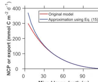
ap-proximation accuracy of Eq. (15), we compare the upper bounds estimated from Eq. (16) and the original model (Eqs. 8–10). Our comparison suggests that the approxima-tion of Eq. (15) is accurate for the estimaapproxima-tion of NCP∗under most conditions (Fig. 3).
We first need to derive the C∗ that maximizes NCP(0, MLD) (i.e., NCP∗) in Eq. (16). C∗ can be solved from the first derivative of NCP(0, MLD) in Eq. (16) with respect toC:
dNCP(0,MLD)
dC
NCP
(0,MLD)=NCP∗
=µ∗· K
w I kc·C∗+KIw
2
−MLD·rHR=0 (17)
and therefore
C∗= 1 kc ·
−KIw+ s
µ∗·KIw
MLD·rHR
. (18)
Equation (18) decreases with MLD. AsC∗is positive (C∗≥
0) and cannot go to infinity (C∗≤Cmax∗ ), MLD should sat-isfy MLDC∗
max≤MLD≤
µ∗
rHR·KIw, where MLDC ∗
maxrepresents
the MLD corresponding to the maximum achievable au-totroph biomass concentration (Cmax∗ ) in the surface ocean. The NCP∗model for 0≤MLD<MLDC∗
max is not discussed
here because we do not have data with very shallow MLD to constrain and evaluate the model. The derivation of the model is, however, presented in the Supplement. Substitut-ingC∗from Eq. (18) into (16) results in
√
NCP∗=a2·p−ln(1−Im(0))+a1· √
MLD, (19)
where a1= −
q
Kw
I ·rHR
kc and a2=
q
Nm·µmax
kc . Constants a1
anda2are functions ofrHRandµmax, respectively, which are
generally modeled to increase with temperature (T) (Eppley, 1972; Rivkin and Legendre, 2001):
µmax=µ0max·ePt·T, (20a)
rHR=rHR0 ·eBt
·T, (20b)
0 30 60 90 120
Mixed layer depth (m) 0
100 200 300 400
NCP or export (mmol C m
-2 d -1)
Original model
[image:5.612.346.508.69.205.2]Approximation using Eq. (15)
Figure 3.Upper bounds derived using the original and approxi-mated models. The upper bound for the original model (Eqs. 8– 10) is estimated through a nonlinear optimization approach. The upper bound for the approximated model is calculated analytically from Eq. (19). The models use the constants listed in Table 1 and
Im(0)=0.9. DecreasingIm(0)and increasingrHRresults in greater
discrepancies between the original and approximated models in re-gions with shallow mixed layers.
wherePt andBt are constants, and µ0max and rHR0 are the
maximum growth rate and heterotrophic respiration ratio for
T =0◦C, respectively. Pt is commonly assumed to equal
0.0663 (Eppley, 1972). Substituting Eqs. (20a) and (20b) into Eq. (19) yields
√
NCP∗=a4·
p
ePt·T ·p−ln(1−Im(0)) +a3·peBt·T·
√
MLD, (21)
wherea3= −
r
rHR0 ·KIw
kc anda4=
q
µ0
max·Nm
kc .
2.5 Comparison to observations 2.5.1 Data products
We assess the performance of our modeled upper bound on carbon export using a global dataset of MLD, PAR, sea surface temperature (SST), O2/ Ar-derived NCP, and export
production derived from sediment traps and234Th (see the Supplement). MLD was derived from global Argo profiles (Global Ocean Data Assimilation Experiment; http://www. usgodae.org/) and CTD casts (National Oceanographic Data Center; https://www.nodc.noaa.gov/). PAR was downloaded from the NASA ocean color website (https://oceancolor.gsfc. nasa.gov/). The NCP estimates are based on a compilation of O2/ Ar measurements from Li and Cassar (2016), Li et
0 30 60 90 120
Mixed layer depth (m)
0 50 100 150
NCP or export (mmol C m
-2 d -1)
max=1, rHR=0.1
max=1.2, rHR=0.2
max=1.2, rHR=0.1
POC export (literature) O2 / Ar-derived NCP
30
20
10
0 SST (
oC)
0 20 40 0
60 80
50
NCP (mmol C m
-2 d -1 )
Mixed layer depth (m)
100 150
0 0.2 0.4 0.6 0.8 >1
NCP
/upper bound
0 5 10 15 20 25 30
SST (oC)
0 50 100 150
NCP (mmol C m
-2 d
-1) 5m
15m
25m
35m 45m 55m
65m 0
20 40 60 80
Mixed layer depth (m)
Upper bound O2 / Ar-derived NCP
(a) (b)
[image:6.612.131.468.65.336.2](c)
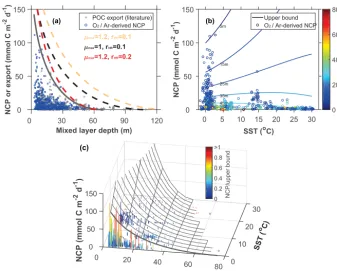
Figure 4.Modeled upper bound on carbon export production compared to field observations as a function of mixed layer depth (MLD) and sea surface temperature (SST).(a)The thick gray line represents the upper bound fitted to the net community production (NCP) data. Dashed lines represent the upper bounds calculated using parameters available in the literature (Table 1).(b)NCP as a function of SST with isopleths of constant upper bounds color coded for MLD. NCP observations are color coded with MLD.(c)Surface representing the envelope of the modeled upper bound of carbon export production as a function of SST and MLD. Bars represent field observations color coded with the ratio of NCP to the upper bound. Observations are based on234Th and sediment trap estimates of carbon export production and O2/ Ar-derived
NCP. A stoichiometric ratio of O2/ C=1.4 was used to convert NCP from O2to C units (Laws, 1991). To account for the effect of PAR on
export production, both MLD and carbon fluxes are normalized to−log(1−Im(0))(see Eqs. 19 and 21). The temperature dependence of
rHRwas modeled asrHR=rHR0 ·e0.08·T.
in Eq. (10) were derived assuming a carbon to chlorophylla
ratio of 90 (Arrigo et al., 2008) and an empirical linear re-lationship between KIand chlorophylla concentration (see Fig. S3 in the Supplement) calculated based on the NOMAD dataset (Werdell and Bailey, 2005). The kmI value was set at 4.1 einstein m−2d−1following Behrenfeld and Falkowski
(1997). In our estimation of the upper bound on carbon ex-port, we setNmto 1 in the NCP∗calculations.
2.5.2 Results and discussion
Overall, we find that NCP∗ calculated using published pa-rameters (Table 1) does a good job of enveloping the carbon export observations reported in the literature (Fig. 4a). Sam-ples on the NCP∗ envelope (upper bound) are likely regu-lated by light availability. Conversely, points below the up-per bound may be nutrient limited. As expected, NCP∗ in-creases with µmaxand decreases withrHR. Model
parame-tersa1= −1.78 anda2=14.75 (Eq. 19) provide the best fit
to the upper bound of O2/ Ar NCP as a function of MLD.
When compared to parameters available in the literature
(Ta-ble 1), we find the best fit to our modeled upper bound when usingµmaxandrHRof 1.2 and 0.2 d−1, respectively. When accounting for the effect ofT onµmaxandrHR, model con-stantsa3= −1.53 anda4=13.39 (Eq. 21) best fit the upper bound on O2/ Ar NCP, SST, and MLD observations.
Our results show that NCP∗decreases faster with increas-ing MLD in warmer waters (Fig. 4b and c) because the terma3·
√
eBt·T in Eq. (21) is negative and negatively
cor-related with T. This temperature effect contributes to part of the relationship between export production and MLD in Fig. 4a. Interestingly, NCP∗increases withT in colder wa-ters and shallow mixed layers (Fig. 4c). This is because NCP∗reflects the balance between productivity (a4·
√ ePt·T· √
−ln(1−Im(0))) and heterotrophic respiration (a3· √
eBt·T· √
MLD). In a shallow, cold mixed layer, the change in pro-ductivity withT (d
a4·
√
ePt·T·√−ln(1−I
m(0))
dT =
Pt
2·a4· √
ePt·T· √
−ln(1−Im(0)))is greater than that of heterotrophic
respi-ration (d
a3·
√
eBt·T·√MLD
dT =
Bt
2 ·a3· √
eBt·T· √
Table 1.Value or range of values with references for the parameters used in the model.
Parameter Range or value Reference
KIw 0.09 Werdell and Bailey (2005)
kc 0.03 Werdell and Bailey (2005)
Carbon to chlorophyll ratio 90 Arrigo et al. (2008)
kmI 4.1 einstein m−2d−1 Behrenfeld and Falkowski (1997)
Pt 0.0663 Eppley (1972)
Bt 0.08 Rivkin and Legendre (2001), López-Urrutia et al. (2006)
µmax 1 d−1, 1.2 d−1 Laws et al. (2000), Eppley (1972)
rHR 0.1 d−1, 0.2 d−1 Laws et al. (2000), Mitchell et al. (1991)
between NCP and SST reported in previous studies (Li and Cassar, 2016). Our NCP∗ model does not perform as well in warmer, deep mixed layers where high variability in ex-port ratio maxima have also been reex-ported (Cael and Fol-lows, 2016). This may stem from uncertainties in observa-tions, the differing relationship betweenT,µmax, andrHRat
high temperature, and/or violations of our assumptions (see the “Caveats and limitations” section).
Several recent studies have explored the relationship of NCP to oceanic parameters based on various statistical ap-proaches (Cassar et al., 2015; Chang et al., 2014; Huang et al., 2012; Li and Cassar, 2016; Li et al., 2016). Our model can shed some light onto the mechanisms driving some of these patterns. To that end, we substitute Eq. (9) into Eq. (8): NCP(0,MLD)=C·MLD
·
−Nm·µmax KI·MLD
·ln I
0·e−KI·MLD+kIm I0+kmI
−rHR
. (22)
Rearranging Eq. (22) results in
NCPB=
NCP(0,MLD) C·MLD = −
lnI0·e−KI·MLD+kmI
I0+kmI
I0· 1−e−KI·MLD
·Nm·µmax·PARML−rHR, (23)
where NCPB is the biomass-normalized volumetric NCP,
PARML is the average PAR in the mixed layer (PARML= 1−e−KI·MLD
KI·MLD ·I0), and− ln
I0·e−KI·MLD+kI m I0+kmI
I0·(1−e−KI·MLD)
·Nm·µmaxand−rHR
correspond to the slope and offset, respectively. The scatter in the relationship between chlorophyll-normalized volumet-ric NCP and PARML, as reported in previous studies (Bender
et al., 2016), can likely be explained by the effect of temper-ature and the availability of nutrients and light (among other properties) on the slope and offset of Eq. (23). Equation (22) can also be reorganized to assess how environmental condi-tions may impact the export ratio (ef):
ef=NCP(0,MLD)
NPP(0,MLD) =1−
KI·MLD
−lnI0·e−KI·MLD+kIm
I0+kIm
· 1
Nm · rHR
µmax
, (24)
where rHR
µmax is proportional to e
(Bt−Pt)·T. Equation (24) is
consistent with multiple studies that predict decreasing ef with increasing temperature (Cael and Follows, 2016; Dunne et al., 2005; Henson et al., 2011; Laws et al., 2000; Li and Cassar, 2016). In fact, Eq. (5) of Cael and Follows (2016) can easily be derived from Eq. (24) (see the Supplement). Equation (24) also highlights the fact that a multitude of fac-tors may confound the dependence of ef on temperature (in-cluding varying MLD, light attenuation, and availability of nutrients and light). This again may explain some of the con-flicting observations recently reported in the literature (e.g., Maiti et al., 2013); the effect of temperature may be masked by changes in community composition (Britten et al., 2017; Henson et al., 2015). One therefore needs to account or cor-rect for the multitude of confounding factors when predicting the effect of a given environmental condition (e.g., tempera-ture, mineral ballast, and NPP) on the export ratio.
3 Spatial distribution of the upper bound on carbon export
We estimate the global distribution of the upper bound of car-bon export using Eq. (19) and climatological monthly MLD and PAR. In general, NCP∗is high in low latitudes and low in the North Atlantic and Antarctic Circumpolar Current (ACC) in the Southern Ocean (Fig. 5a). As expected, this spatial pat-tern is controlled by MLD (see Fig. S1). Satellite-derived estimates of NCP (Li and Cassar, 2016) are approximately 10 % of global NCP∗, reflecting the high degree of nutrient limitation in the oceans. We also derive a global NCP∗map using Eq. (21) and find that the global NCP∗estimate is very sensitive to the temperature dependence ofrHR. For
exam-ple, decreasing theBtinrHR=rHR0 ·eBt
·T from 0.11 to 0.08
Annual
180o W 90oW 0o 90o E 180o W 90oS
45oS 0o 45 N o 90 N o
0 20 40 60 80 100
Export potential (mol C m -2 yr -1)
Annual
90oS 45oS 0o 45oN 90oN
0 0.2 0.4 0.6 0.8 1
NCP/NCP
*
Spring
90oS 45oS 0o 45oN 90oN
0 0.2 0.4 0.6 0.8 1
NCP/NCP
* Summer
90oS 45oS 0o 45oN 90oN
0 0.2 0.4 0.6 0.8 1
NCP/NCP
*
Summer
90oS 45oS 0o 45oN 90oN
0 0.2 0.4 0.6 0.8 1
Bio. pump efficiency
Summer
90oS 45oS 0o 45oN 90oN
0 0.2 0.4 0.6 0.8 1
Export ratio
80o W 90o W 0o 90o E 180o W 1
80o W 90oW 0o 90o E 180o W
1 180oW 90o W 0o 90oE 180oW 80oW 90oW 0o 90oE 180oW 1
80oW 90o W 0o 90oE 180oW 1
(a) (b)
(c) (d)
(e) (f)
Figure 5. (a)Modeled upper bound on carbon export derived from Eq. (19),(b–d)ratios of satellite export production estimates to the upper bound on carbon export,(e)biological pump efficiency calculated as the difference in nutrient concentrations between surface and depth normalized to nutrient concentrations at depth (Sarmiento and Gruber, 2006; nitrate concentration from the World Ocean Atlas at https://www.nodc.noaa.gov/OC5/woa13/), and(f)export ratio derived from Dunne et al. (2005). “Annual” represents the annually integrated value. Spring and summer represent the average value in spring and summer, respectively. In the Northern Hemisphere, the spring and summer seasons are defined as March–May and June–August, respectively. In the Southern Hemisphere, the spring and summer seasons are defined as September–November and December–February, respectively.
López-Urrutia et al., 2006), we hereafter only discuss NCP∗ estimates derived from Eq. (19).
To estimate how close export production is to its upper bound, we calculate the ratio of export production to NCP∗ (fpt). Low fpt regimes represent ecosystems likely
regu-lated by nutrient availability (i.e., ecosystems that have not reached their full export potential based on MLD and sur-face PAR). As expected, low-latitude and subtropical regions have low fpt (Fig. 5b). Highfpt regimes represent
ecosys-tems that have reached their full light potential and are there-fore less likely to respond to nutrient addition because of light limitation (e.g., the North Atlantic and ACC; Fig. 5b). In these regions, especially the subantarctic region,fpt is high in the spring (Fig. 5c) and decreases in the summer (Fig. 5d), suggesting that export production is likely co-limited by nu-trient and light availability. This may in part explain the lower response to iron fertilization in the subantarctic region where substantial increases in surface chlorophyll were only observed in regions with shallower mixed layers (Boyd et al., 2007, 2000; de Baar et al., 2005).
Also shown in Fig. 5 are the biological pump efficiency and export ratios (Fig. 5e and f, respectively). These various proxies reflect different components of the biological pump. Whereas fpt reflects the export potential based on current
MLD and light availability, the biological pump efficiency
reflects the potential as derived from nutrient distribution in the oceans and estimated from the extent of nutrient removal from the surface ocean (Sarmiento and Gruber, 2006) or the proportion of regenerated nutrients at depth (Ito and Follows, 2005). A revised estimate of the global biological pump ef-ficiency, estimated based on the proportion of regenerated to total nutrients (preformed+regenerated) at depth, is around 30–35 % (Duteil et al., 2013). The ef ratio, however, de-scribes how much of production is exported as opposed to re-cycled in the surface (Dunne et al., 2005). Ultra-oligotrophic subtropical waters have a low export ratio and a strong bi-ological pump efficiency with exhaustion of nutrients at the ocean surface; they have therefore not reached their full light potential (low fpt) because of the strong stratification and nutrient limitation. The seasonal pattern of fpt in the sub-antarctic region suggests that low biological pump efficiency is the result of light limitation in the austral spring and nutri-ent (likely Fe) and light limitation in the austral summer.
4 Caveats and limitations
[image:8.612.116.482.66.307.2]– In our study, we used a model that builds on Sver-drup’s critical depth hypothesis. There are competing hypotheses to explain phytoplankton bloom phenology (timing and intensity), including the “dilution recou-pling hypothesis” or “disturbance recovery hypothe-sis” (Behrenfeld, 2010; Boss and Behrenfeld, 2010) and the “critical turbulence hypothesis” (Brody and Lozier, 2015; Huisman et al., 1999; Taylor and Ferrari, 2011). In the case of top-down control, any respiratory graz-ing loss not accounted for by our loss term would behave as a system not reaching its full light poten-tial (NCP∗). Conversely, any grazing loss associated with export (e.g., rapidly sinking fecal pellets and other zooplankton-mediated export pathways) would mini-mize respiratory losses, thereby bringing NCP closer to its upper bound based on light availability. These oppos-ing effects are beyond the scope of this study but could be modeled, especially as we learn more about their im-pacts on carbon fluxes through new efforts such as the NASA EXPORTS program (Siegel et al., 2016). See also the point below on mixing vs. mixed layer depth. – Phytoplankton biomass concentration (C) may vary
with depth in the mixed layer, especially for water columns experiencing varying degrees of turbulent mix-ing. In addition, MLD is not always the best proxy for light availability with the mixing layer in some cases deviating from the mixed layer (Franks, 2015; Huisman et al., 1999). The factors defining the MLD also vary in different oceanic regions.
– For simplicity, we model the dependence of photosyn-thesis on irradiance assuming Michaelis–Menten kinet-ics, which does not account for photoinhibition. More accurate models can be found in other studies (Platt et al., 1980). Due to optional absorption, KI also varies
with depth in the mixed layer. Additionally, the linear relationship betweenKIandCis influenced by CDOM,
NAP, and other environmental factors (e.g., solar zenith angle; Gordon, 1989).
– TheµmaxandrHRvalues are influenced by
environmen-tal factors other than temperature, including community structure (Chen and Laws, 2017), and may vary with depth within the mixed layer (Smetacek and Passow, 1990). For these reasons, the equations relating µmax
andrHR(i.e.,Bt andPt) to temperature also carry
sig-nificant uncertainties (Bissinger et al., 2008; Edwards et al., 2016; Kremer et al., 2017; López-Urrutia and Morán, 2007; Rivkin and Legendre, 2001), which im-pacts our estimates of the upper bound on carbon ex-port, especially in warmer regions. As in other recent studies (Cael and Follows, 2016; Cael et al., 2017; Dutkiewicz et al., 2001; Gong et al., 2015, 2017; Huis-man et al., 2006; Taylor and Ferrari, 2011), we model heterotrophic respiration to vary in proportion to
phy-toplankton concentration. The model could be further improved by explicitly including the concentration of heterotrophs. See the point above on the grazing effect on export with regards torHR.
– NCP may underestimate export production when ac-companied by a decrease in the inventory of organic matter in the mixed layer (see the Introduction and Eq. 2).
– Our field observations are limited, mostly focusing on the spring and summer seasons, and harbor significant uncertainties. For example, deep mixed layers can bias the O2/ Ar method low if entrainment of deeper
wa-ters brings low O2into the mixed layer. Descriptions of
these uncertainties are presented in other studies (Ben-der et al., 2011; Cassar et al., 2014; Jonsson et al., 2013). – Finally, our study is only relevant to the mixed layer. It does not account for productivity below the mixed layer, which can be important in some regions such as the subtropical ocean.
5 Conclusions
In this study, we derived a mechanistic model of an upper bound on carbon export (NCP∗) based on the metabolic bal-ance between photosynthesis and respiration of the plank-ton community. The upper bound is a positively skewed bell-shaped function of mixed layer depth (MLD). At low temper-atures, the upper bound decreases with temperature if mixed layers are deep, but increases with temperature if mixed lay-ers are shallow. We used this model to derive a global dis-tribution of an upper bound on carbon export as a function of MLD and surface PAR, which shows high values in low latitudes and low values in high latitudes due to deep MLD. To examine how current export production compares to this upper bound in the world’s oceans, we calculated the ratio of satellite export production estimates to the upper bound de-rived by our model. High ratios of export production to NCP∗ in the North Atlantic and ACC indicate that export produc-tion in these regions is likely co-limited by nutrient and light availability. Overall, our results may explain the differences in carbon export measured during past iron fertilization ex-periments (e.g., subantarctic and polar regions), inform fu-ture iron fertilization experiments, help in the development of remotely sensed carbon export algorithms, and improve predictions of the response of marine ecosystems to a chang-ing climate.
Data availability. Our O2/Ar measurements can be downloaded
Appendix A: Model symbols, abbreviations, and units
Symbol Description Units
MLD Mixed layer depth m
MLDC∗
max Maximum MLD corresponds to maximum achievable autotroph biomass concentration m
z Depth m
Zc Critical depth m
Zp Compensation depth m
GPP(0,z) Gross primary production mmol C m−2d−1
NPP(z) Net primary production at depthz mmol C m−3d−1
NPP(0,z) Net primary production above depthz mmol C m−2d−1
NCP(z) Net community production at depthz mmol C m−3d−1
NCP(0,z) Net community production above depthz mmol C m−2d−1
HR(z) Heterotrophic respiration at depthz mmol C m−3d−1
HR(0,z) Heterotrophic respiration above depthz mmol C m−2d−1
NCP∗ The maximum NCP for a given MLD (upper bound on carbon export) mmol C m−2d−1
NCPB NCP normalized to autotroph biomass inventory in the mixed layer d−1
ef Export ratio unitless
fpt Ratio of satellite export production estimates to the upper bound on carbon export unitless
N Nutrient concentration mmol m−3
kNm Half-saturation constant for nutrient concentration mmol m−3
Nm Nutrient effect on phytoplankton growthNm=N+NkN
m unitless
PAR Photosynthetically active radiation einstein m−2d−1
I0 Photosynthetically active radiation just beneath water surface einstein m−2d−1
I (z) Photosynthetically active radiation at depthz einstein m−2d−1
kI
m Half-saturation constant for irradiance einstein m−2d−1
Im(z) Light effect on phytoplankton growth at depthz,Im(z)=I (z)I (z)+kI m
= I0·e−KI·z I0·e−KI·z+kI
m
unitless
Im(0, z) Integrated light effect on phytoplankton growth above depthz,Im(0, z)= −KI1 ·ln
I0·e−KI·z+kI m I0+kI
m
unitless
PARML Average PAR in the mixed layer (PARML=1−e −KI·MLD
KI·MLD ·I0) einstein m
−2d−1
µ Phytoplankton growth rate d−1
µmax Maximum phytoplankton growth rate d−1
µ0max Maximum phytoplankton growth rate forT =0◦C d−1
rHR Heterotrophic respiration ratio d−1
rHR0 Heterotrophic respiration ratio forT =0◦C d−1
KI Light attenuation coefficient (KI=KIw+KInw) m−1
KIw Light attenuation coefficient due to water m−1
KInw Light attenuation coefficient due to optically active components m−1
kc Specific attenuation coefficient for irradiance m2mmol−1
C Phytoplankton biomass concentration mmol m−3
C∗ Phytoplankton biomass concentration that maximizes NCP mmol m−3
Cmax∗ Maximum achievable autotroph biomass concentration mmol m−3
POC Particulate organic carbon mmol m−3
DOC Dissolved organic carbon mmol m−3
CDOM Colored dissolved organic matter m−1
NAP Non-algal particles mmol m−3
T Temperature ◦C
Pt Temperature dependence for phytoplankton growth rate ◦C−1
Bt Temperature dependence for heterotrophic respiration ratio ◦C−1
The Supplement related to this article is available online at https://doi.org/10.5194/bg-14-5015-2017-supplement.
Competing interests. The authors declare that they have no conflict of interest.
Acknowledgements. We would like to acknowledge NASA
GSFC for processing and distributing PAR and SST
products (http://oceancolor.gsfc.nasa.gov/). Global Argo temperature–salinity profiling floats were downloaded from http://www.usgodae.org/. CTD casts were downloaded from the Na-tional Oceanographic Data Center (https://www.nodc.noaa.gov/). NC was supported by NSF OPP-1043339. ZL was supported by a NASA Earth and Space Science Fellowship (grant no. NNX13AN85H). The authors thank three anonymous reviewers for their insightful comments.
Edited by: Jack Middelburg
Reviewed by: three anonymous referees
References
Arrigo, K. R., van Dijken, G. L., and Bushinsky, S.: Primary pro-duction in the Southern Ocean, 1997–2006, J. Geophys. Res., 113, C08004, https://doi.org/10.1029/2007JC004551, 2008. Baker, K. S. and Smith, R. C.: Bio-optical classification and
model of natural waters. 2, Limnol. Oceanogr., 27, 500–509, https://doi.org/10.4319/lo.1982.27.3.0500, 1982.
Behrenfeld, M. J.: Abandoning Sverdrup’s Critical Depth Hy-pothesis on phytoplankton blooms, Ecology, 91, 977–989, https://doi.org/10.1890/09-1207.1, 2010.
Behrenfeld, M. J. and Falkowski, P. G.: Photosynthetic rates de-rived from satellite-based chlorophyll concentration, Limnol. Oceanogr., 42, 1–20, https://doi.org/10.4319/lo.1997.42.1.0001, 1997.
Bender, M. L., Tilbrook, B., Cassar, N., Jonsson, B. F., Poisson, A., and Trull, T. W.: Ocean productivity south of Australia during spring and summer, Deep-Sea Res. Pt. I, 112, 68–78, https://doi.org/10.1016/j.dsr.2016.02.018, 2016.
Bender, M. L., Kinter, S., Cassar, N., and Wanninkhof, R.: Evaluating gas transfer velocity parameterizations us-ing upper ocean radon distributions, J. Geophys. Res., 116, https://doi.org/10.1029/2009JC005805, 2011.
Bissinger, J. E., Montagnes, D. J. S., Sharples, J., and Atkin-son, D.: Predicting marine phytoplankton maximum growth rates from temperature: Improving on the Eppley curve us-ing quantile regression, Limnol. Oceanogr., 53, 487–493, https://doi.org/10.4319/lo.2008.53.2.0487, 2008.
Boss, E. and Behrenfeld, M. J.: In situ evaluation of the initiation of the North Atlantic phytoplankton bloom, Geophys. Res. Lett., 37, https://doi.org/10.1029/2010GL044174, 2010.
Boyd, P. W., Jickells, T., Law, C. S., Blain, S., Boyle, E. A., Buesseler, K. O., Coale, K. H., Cullen, J. J., de Baar, H. J. W., Follows, M., Harvey, M., Lancelot, C., Levasseur, M.,
Owens, N. P. J., Pollard, R., Rivkin, R. B., Sarmiento, J., Schoe-mann, V., Smetacek, V., Takeda, S., Tsuda, A., Turner, S., and Watson, A. J.: Mesoscale iron enrichment experiments 1993– 2005: Synthesis and future directions, Science, 315, 612–617, https://doi.org/10.1126/science.1131669, 2007.
Boyd, P. W., Watson, A. J., Law, C. S., Abraham, E. R., Trull, T., Murdoch, R., Bakker, D. C. E., Bowie, A. R., Buesseler, K. O., Chang, H., Charette, M., Croot, P., Downing, K., Frew, R., Gall, M., Hadfield, M., Hall, J., Harvey, M., Jameson, G., LaRoche, J., Liddicoat, M., Ling, R., Maldonado, M. T., McKay, R. M., Nodder, S., Pickmere, S., Pridmore, R., Rintoul, S., Safi, K., Sut-ton, P., Strzepek, R., Tanneberger, K., Turner, S., Waite, A., and Zeldis, J.: A mesoscale phytoplankton bloom in the polar South-ern Ocean stimulated by iron fertilization, Nature, 407, 695–702, https://doi.org/10.1038/35037500, 2000.
Britten, G. L., Wakamatsu, L., and Primeau, F. W.: The temperature-ballast hypothesis explains carbon export efficiency observations in the Southern Ocean, Geophys. Res. Lett., 44, 1831–1838, https://doi.org/10.1002/2016GL072378, 2017.
Brody, S. R. and Lozier, M. S.: Characterizing upper-ocean mixing and its effect on the spring phytoplankton bloom with in situ data, ICES J. Mar. Sci., 72, 1961–1970, https://doi.org/10.1093/icesjms/fsv006, 2015.
Cael, B. B. and Follows, M. J.: On the temperature dependence of oceanic export efficiency, Geophys. Res. Lett., 43, 5170–5175, https://doi.org/10.1002/2016GL068877, 2016.
Cael B. B., Bisson, K., and Follows, M. J.: How have re-cent temperature changes affected the efficiency of ocean biological carbon export?, Limnol. Oceanogr., 2, 113–118, https://doi.org/10.1002/lol2.10042, 2017.
Cassar, N., Nevison, C. D., and Manizza, M.: Correcting oceanic O2/Ar-net community production estimates for vertical mixing
using N2O observations, Geophys. Res. Lett., 41, 8961–8970,
https://doi.org/10.1002/2014GL062040, 2014.
Cassar, N., DiFiore, P. J., Barnett, B. A., Bender, M. L., Bowie, A. R., Tilbrook, B., Petrou, K., Westwood, K. J., Wright, S. W., and Lefevre, D.: The influence of iron and light on net com-munity production in the Subantarctic and Polar Frontal Zones, Biogeosciences, 8, 227–237, https://doi.org/10.5194/bg-8-227-2011, 2011.
Cassar, N., Wright, S. W., Thomson, P. G., Trull, W. T., West-wood, K. J., de Salas, M., Davidson, A., Pearce, I., Davies, D. M., and Matear, R. J.: The relation of mixed-layer net com-munity production to phytoplankton comcom-munity composition in the Southern Ocean, Global Biogeochem. Cy., 29, 446-462, https://doi.org/10.1002/2014GB004936, 2015.
Chang, C.-H., Johnson, N. C., and Cassar, N.: Neural network-based estimates of Southern Ocean net community pro-duction from in situ O2/Ar and satellite observation:
a methodological study, Biogeosciences, 11, 3279–3297, https://doi.org/10.5194/bg-11-3279-2014, 2014.
Chen, B. and Laws, E. A.: Is there a difference of temperature sen-sitivity between marine phytoplankton and heterotrophs?, Lim-nol. Oceanogr., 62, 806–817, https://doi.org/10.1002/lno.10462, 2017.
de Barr, J. W. H., Boyd, P. W., Coale, K. H., Landry M. R., Tsuda, A., Assmy, P., Bakker, D. C. E., Bozec, Y., Barber, R. T., Brzezinski, M. A., Buesseler, K. O., Boyé, M., Croot, P. L., Gervais, F., Gorbunov, M. Y., Harrison, P. J., Hiscock, W. T., Laan, P., Lancelot, C., Law, C. S., Levasseur, M., Marchetti, A., Millero, F. J., Nishioka, J., Nojiri, Y., van Oijen, T., Riebe-sell, U., Rijkenberg, M. J. A., Saito, H., Takeda, S., Timmer-mans, K. R., Veldhuis, M. J. W., Waite, A. M., and Wong, C. S.: Synthesis of iron fertilization experiments: From the Iron age in the Age of Enlightenment, J. Geophys. Res., 110, C09S16, https://doi.org/10.1029/2004JC002601, 2005.
Dunne, J. P., Armstrong, R. A., Gnanadesikan, A., and Sarmiento, J. L.: Empirical and mechanistic models for the particle export ratio, Global Biogeochem. Cy., 19, https://doi.org/10.1029/2004GB002390, 2005.
Duteil, O., Koeve, W., Oschlies, A., Bianchi, D., Galbraith, E., Kri-est, I., and Matear, R.: A novel estimate of ocean oxygen utilisa-tion points to a reduced rate of respirautilisa-tion in the ocean interior, Biogeosciences, 10, 7723–7738, https://doi.org/10.5194/bg-10-7723-2013, 2013.
Dutkiewicz, S., Follows, M., Marshall, J., and Gregg, W. W.: Interannual variability of phytoplankton abundances in the North Atlantic, Deep-Sea Res. Pt. II, 48, 2323–2344, https://doi.org/10.1016/S0967-0645(00)00178-8, 2001. Edwards, K. F., Thomas, M. K., Klausmeier, C. A., and Litchman,
E.: Phytoplankton growth and the interaction of light and temper-ature: A synthesis at the species and community level, Limnol. Oceanogr., 61, 1232–1244, https://doi.org/10.1002/lno.10282, 2016.
Eppley, R. W.: Temperature and phytoplankton growth in the sea, Fish. B.-NOAA, 70, 1063–1085, 1972.
Eveleth, R., Cassar, N., Sherrell, R. M., Ducklow, H., Mered-ith, M., Venables, H., Lin, Y., and Li, Z.: Ice melt influence on summertime net community production along the West-ern Antarctic Peninsula, Deep-Sea Res. Pr. II, 139, 89-102, https://doi.org/10.1016/j.dsr2.2016.07.016, 2017.
Falkowski, P. G., Barber, R. T., and Smetacek, V.: Biogeochemical controls and feedbacks on ocean primary production, Science, 281, 200-206, https://doi.org/10.1126/science.281.5374.200, 1998.
Franks, P. J. S.: Has Sverdrup’s critical depth hypothesis been tested? Mixed layers vs. turbulent layers, ICES J. Mar. Sci., 72, 1897–1907, https://doi.org/10.1093/icesjms/fsu175, 2015. Gong, X., Shi, J., Gao, H. W., and Yao, X. H.: Steady-state
so-lutions for subsurface chlorophyll maximum in stratified water columns with a bell-shaped vertical profile of chlorophyll, Bio-geosciences, 12, 905–919, https://doi.org/10.5194/bg-12-905-2015, 2015.
Gong, X., Jiang, W., Wang, L., Gao, H., Boss, E., Yao, X., Kao, S., and Shi, J.: Analytical solution of the nitra-cline with the evolution of subsurface chlorophyll maximum in stratified water columns, Biogeosciences, 14, 2371–2386, https://doi.org/10.5194/bg-14-2371-2017, 2017.
Gordon, H. R.: Can the Lambert-Beer law be applied to the diffuse attenuation coefficient of ocean water? Limnol. Oceanogr., 34, 1389–1409, https://doi.org/10.4319/lo.1989.34.8.1389, 1989. Henson, S. A., Yool, A., and Sanders, R.:
Variabil-ity in efficiency of particulate organic carbon export:
A model study, Global Biogeochem. Cy., 29, 33–45, https://doi.org/10.1002/2014GB004965, 2015.
Henson, S. A., Sanders, R., Madsen, E., Morris, P. J., Le Moigne, F., and Quartly, G. D.: A reduced estimate of the strength of the ocean’s biological carbon pump, Geophys. Res. Lett., 38, L04606, https://doi.org/10.1029/2011GL046735, 2011. Huang, K., Ducklow, H., Vernet, M., Cassar, N., and
Ben-der, M. L.: Export production and its regulating fac-tors in the West Antarctica Peninsula region of the Southern Ocean, Global Biogeochem. Cy., 26, GB2005, https://doi.org/10.1029/2010GB004028, 2012.
Huisman, J. and Weissing, F. J.: Light-limited growth and competi-tion for light in well-mixed aquatic environments: An elementary model, Ecology, 75, 507–520, https://doi.org/10.2307/1939554, 1994.
Huisman, J., van Oostveen, P., and Weissing, F. J.: Critical depth and critical turbulence: Two different mechanisms for the devel-opment of phytoplankton blooms, Limnol. Oceanogr., 44, 1781– 1787, https://doi.org/10.4319/lo.1999.44.7.1781, 1999.
Huisman, J., Thi, N. N. P., Karl, D. M., and Sommeijer B.: Reduced mixing generates oscillations and chaos in the oceanic deep chlorophyll maximum, Nature, 439, 322–325, https://doi.org/10.1038/nature04245, 2006.
Ito, T. and Follows, M. J.: Preformed phosphate, soft tissue pump and atmospheric CO2, J. Mar. Res., 63, 813–839,
https://doi.org/10.1357/0022240054663231, 2005.
Jonsson, B. F., Doney, S. C., Dunne, J., and Bender, M.: Eval-uation of the Southern Ocean O2/Ar-based NCP estimates in a model framework, J. Geophys. Res., 118, 385–399, https://doi.org/10.1002/jgrg.20032, 2013.
Kremer, C. T., Thomas, M. K., and Litchman, E.: Temperature-and size-scaling of phytoplankton population growth rates: Reconciling the Eppley curve and the metabolic theory of ecology, Limnol. Oceanogr., 62, 1658–1670, https://doi.org/10.1002/lno.10523, 2017.
Laws, E. A., Falkowski, P. G., Smith, W. O., Ducklow, H., and McCarthy, J. J.: Temperature effects on export production in the open ocean, Global Biogeochem. Cy., 14, 1231–1246, https://doi.org/10.1029/1999GB001229, 2000.
Lewis, M. R., Cullen, J. J., and Platt, T.: Relationships be-tween vertical mixing and photoadaptation of phytoplank-ton: Similarity criteria, Mar. Ecol. Prog. Ser., 15, 141–149, https://doi.org/10.3354/meps015141, 1984.
Li, Z. and Cassar, N.: Satellite estimates of net commu-nity production based on O2/Ar observations and
compari-son to other estimates, Global Biogeochem. Cy., 30, 735–752, https://doi.org/10.1002/2015GB005314, 2016.
Li, Z., Cassar, N., Huang, K., Ducklow, H., and Schofield, O.: In-terannual variability in net community production at the Western Antarctic Peninsula region (1997–2014), J. Geophys. Res., 121, 4748–4762, https://doi.org/10.1002/2015JC011378, 2016. López-Urrutia, A. and Morán, X. A. G.: Resource
limita-tion of bacterial produclimita-tion distorts the temperature depen-dence of oceanic carbon cycling, Ecology, 88, 817–822, https://doi.org/10.1890/06-1641, 2007.
Maiti, K., Charette, M. A., Buesseler, K. O., and Kahru M.: An inverse relationship between production and export efficiency in the Southern Ocean, Geophys. Res. Lett., 40, 1557–1561, https://doi.org/10.1002/grl.50219, 2013.
Martin, J. H., Knauer, G. A., Karl, D. M., and Broenkow, W. W.: VERTEX: carbon cycling in the northeast Pacific, Deep-Sea Res., 34, 267–285, https://doi.org/10.1016/0198-0149(87)90086-0, 1987.
Martin, P., Rutgers van der Loeff, M., Cassar, N., Vandromme, P., d’Ovidio, F., Stemman, L., Rengarajan, R., Soares, M., Gon-zalez, H. E., Ebersbach, F., Lampitt, R., Sanders, R., Bar-nett, B., Smetacek, V., and Naqvi, S. W. A.: Iron fertiliza-tion enhanced net community producfertiliza-tion but not downward particle flux during the Southern Ocean iron fertilization ex-periment LOHAFEX, Global Biogeochem. Cy., 27, 871–881, https://doi.org/10.1002/gbc.20077, 2013.
Mitchell, B. G. and Holm-Hansen, O.: Observations and modeling of the Antarctic phytoplankton crop in relation to mixing depth, Deep-Sea Res., 38, 981–1007, https://doi.org/10.1016/0198-0149(91)90093-U, 1991.
Mitchell, B. G., Brody, E. A., Holm-Hansen, O., Mc-Clain, C., and Bishop, J.: Light limitation of phyto-plankton biomass and macronutrient utilization in the Southern Ocean, Limnol. Oceanogr., 36, 1662–1677, https://doi.org/10.4319/lo.1991.36.8.1662, 1991.
Morel, A. and Prieur, L.: Analysis of variations
in ocean color, Limnol. Oceanogr., 22, 709–722, https://doi.org/10.4319/lo.1977.22.4.0709, 1977.
Mouw, C. B., Barnett, A., McKinley, G., Gloege, L., and Pilcher, D.: Global ocean particulate organic carbon flux merged with satellite parameters, Earth Syst. Sci. Data, 8, 531–541, https://doi.org/10.5194/essd-8-531-2016, 2016.
Nelson, D. M. and Smith, W. O.: Sverdrup revisited: Crit-ical depths, maximum chlorophyll levels, and the con-trol of Southern Ocean productivity by the irradiance-mixing regime, Limnol. Oceanogr., 36, 1650–1661, https://doi.org/10.4319/lo.1991.36.8.1650, 1991.
Platt, T., Gallegos, C. L., and Harrison, W. G.: Photoinhibition of photosynthesis in natural assemblages of marine phytoplankton, J. Mar. Res., 38, 687–701, 1980.
Rivkin, R. B. and Legendre, L.: Biogenic carbon cycling in the up-per ocean: Effects of microbial respiration, Science, 291, 2398– 2400, https://doi.org/10.1126/science.291.5512.2398, 2001. Sarmiento, J. L. and Gruber, N.: Ocean Biogeochemical Dynamics,
Princeton University Press, Princeton, New Jersey, 2006. Shadwick, E. H., Tilbrook, B., Cassar, N., Trull, T. W.,
and Rintoul, S. R.: Summertime physical and biologi-cal controls on O2 and CO2 in the Australian
Sec-tor of the Southern Ocean, J. Marine Syst., 147, 21–28, https://doi.org/10.1016/j.jmarsys.2013.12.008, 2015.
Siegel, D. A., Buesseler, K. O., Behrenfeld, M. J., Benitez-Nelson, C. R., Boss, E., Brzezinski, M. A., Burd, A., Carlson, C. A., D’Asaro, E. A., Doney, S. C., Perry, M. J., Stanley, R. H. R., and Steinberg, D. K.: Prediction of the export and fate of global ocean net primary production: The exports science plan, Front. Mar. Sci., 3, 22 pp., https://doi.org/10.3389/fmars.2016.00022, 2016.
Sigman, D. M. and Boyle, E. A.: Glacial/interglacial varia-tions in atmospheric carbon dioxide, Nature, 407, 859–869, https://doi.org/10.1038/35038000, 2000.
Smetacek, V. and Passow, U.: Spring bloom initiation and Sver-drup’s critical depth model, Limnol. Oceanogr., 35, 228–234, https://doi.org/10.4319/lo.1990.35.1.0228, 1990.
Smith, R. C. and Baker, K. S.: Optical classification of natural waters, Limnol. Oceanogr., 23, 260–267, https://doi.org/10.4319/lo.1978.23.2.0260, 1978a.
Smith, R. C. and Baker, K. S.: The bio-optical state of ocean waters and remote sensing, Limnol. Oceanogr., 23, 247–259, https://doi.org/10.4319/lo.1978.23.2.0247, 1978b.
Stange, P., Bach, L. T., Le Moigne, F. A. C., Taucher, J., Boxham-mer, T., and Riebesell, U.: Quantifying the time lag between or-ganic matter production and export in the surface ocean: Implica-tions for estimates of export efficiency, Geophys. Res. Lett., 44, 268–276, https://doi.org/10.1002/2016GL070875, 2017. Sunda, W. G. and Huntsman, S. A.: Interrelated influence of iron,
light and cell size on marine phytoplankton growth, Nature, 390, 389–392, https://doi.org/10.1038/37093, 1997.
Sverdrup, H. U.: On conditions for the vernal blooming of phyto-plankton, Journal du Conseil International pour l’Exploration de la Mer, 18, 287–295, https://doi.org/10.1093/icesjms/18.3.287, 1953.
Taylor, J. R. and Ferrari, R.: Shutdown of turbulent con-vection as a new criterion for the onset of spring phy-toplankton blooms, Limnol. Oceanogr., 56, 2293–2307, https://doi.org/10.4319/lo.2011.56.6.2293, 2011.
Tortell, P. D., Bittig, H. C., Körtzinger, A., Jones, E. M., and Hoppema, M.: Biological and physical controls on N2,
O2, and CO2 distributions in contrasting Southern Ocean
surface waters, Global Biogeochem. Cy., 29, 994–1013, https://doi.org/10.1002/2014GB004975, 2015.
Volk, T. and Hoffert, M. I.: Ocean carbon pumps: Analysis of rela-tive strengths and efficiencies in ocean-driven atmospheric CO2 changes, in: The Carbon Cycle and Atmospheric CO2: Natural
Variations Archean to Present, edited by Sundquist, E. T. and Broecker, W. S., AGU, Washington, D. C., Geophys. Monogr. Ser., 32, 99–110, 1985.
Werdell, P. J. and Bailey, S. W.: An improved in-situ bio-optical data set for ocean color algorithm development and satellite data product validation, Remote Sens. Environ., 98, 122–140, https://doi.org/10.1016/j.rse.2005.07.001, 2005.