Computational and theoretical study of the wave-particle interaction of protons and waves

www.ann-geophys.net/30/1361/2012/ doi:10.5194/angeo-30-1361-2012

© Author(s) 2012. CC Attribution 3.0 License.

Annales

Geophysicae

Computational and theoretical study of the wave-particle

interaction of protons and waves

P. S. Moya1, A. F. Vi ˜nas2, V. Mu ˜noz1, and J. A. Valdivia1,3,4

1_{Departamento de F´ısica, Facultad de Ciencias, Universidad de Chile, Las Palmeras 3425, Casilla 653, Santiago, Chile} 2_{NASA Goddard Space Flight Center, Heliophysics Science Division, Geospace Physics Laboratory, Code 673, Greenbelt,} MD 20771, USA

3_{Centro para el Desarrollo de la Nanociencia y Nanotecnolog´ıa, CEDENNA, Chile} 4_{CEIBA complejidad, Carrera 19A 1-37 Este Of. C222, Bogota, Colombia} Correspondence to: P. S. Moya ([email protected])

Received: 20 November 2011 – Revised: 27 April 2012 – Accepted: 23 August 2012 – Published: 19 September 2012

Abstract. We study the wave-particle interaction and the evolution of electromagnetic waves propagating through a plasma composed of electrons and protons, using two ap-proaches. First, a quasilinear kinetic theory has been de-veloped to study the energy transfer between waves and particles, with the subsequent acceleration and heating of protons. Second, a one-dimensional hybrid numerical sim-ulation has been performed, with and without including an expanding-box model that emulates the spherical expansion of the solar wind, to investigate the fully nonlinear evolu-tion of this wave-particle interacevolu-tion. Numerical results of both approaches show that there is an anisotropic evolution of proton temperature.

Keywords. Space plasma physics (Kinetic and MHD the-ory; Numerical simulation studies; Wave-particle interac-tions)

1 Introduction

The problem of acceleration and heating of plasmas due to the interaction of particles with propagating waves has re-ceived special attention during the last decades, especially in the field of laboratory and space plasma physics. In the case of the solar wind (Axford and McKenzie, 1992, 1996; Kohl et al., 1998; Marsch, 1998; Cranmer et al., 1999a,b; Esser et al., 1999; Hu and Habbal, 1999; Tu and Marsch, 1999; Cranmer, 2002), recent observations and theoretical results seem to indicate that most of the acceleration process occurs within a few solar radii from the Sun and the main

mechanism is due to resonant absorption of ion-cyclotron waves (Isenberg, 2001; Cranmer, 2002; Hollweg and Isberg, 2002). However, the detailed processes for the en-ergy transfer between waves and different particle species are still an open question. To address these issues, we in-vestigate the wave-particle interaction and evolution of cir-cularly polarized electromagnetic proton-cyclotron waves propagating parallel to the background magnetic field. Fur-ther studies of the solar wind turbulence in the neighbor-hood of the break of the inertial range spectra as a function of wave vector, with components parallel (kk) and

perpen-dicular (k⊥) to the magnetic field, revealed that the

fluctu-ation spectrum is anisotropic and that the power distribu-tion sometimes is greater at quasi-perpendicular wave vec-tors(k⊥kk)(Matthaeus et al., 1990; Horbury et al., 2005;

Dasso et al., 2005) than at quasi-parallel propagation(kk

k⊥). However, at very long wavelength (smaller k), there

is still enough energy available for the quasi-parallel prop-agating waves to dominate the oblique wave modes (where kkk⊥) (Matthaeus et al., 1990, 1996a,b; Leamon et al.,

2000; Smith et al., 2001, 2006; Horbury et al., 2005, 2008; Bale et al., 2005, 2009), and we focus our study on this part of the wave spectrum range.

nonlinear order in Vlasov’s formalism (Alexandrov et al., 1984; Krall and Trivelpiece, 1986). Second, we performed a one-dimensional hybrid simulation (Gary et al., 1997; Of-man et al., 2001; Araneda et al., 2002) of the system using an expanding box model (Velli et al., 1990; Liewer et al., 2001; Matteini et al., 2006; Hellinger and Tr´avniˇceck, 2008; Ofman et al., 2011) where a thin box of plasma moves away from the Sun in a moving frame at the local solar wind speed, in order to investigate the full nonlinear wave-particle inter-action of the cascade process. All these effects; i.e., energy cascade, expansion, and nonlinear wave-particle interaction, are included in the study to show how the shape of the parti-cle velocity distribution functions is controlled and regulated in kinetic plasmas.

This article is organized as follows. In Sect. 2 we show the basic equations of the quasilinear theory for the evolution of the macroscopic parameters of the distribution function, and we present numerical results for the case of the propa-gation of circularly polarized electromagnetic waves parallel to an ambient magnetic field, through a plasma composed of electrons and protons with thermal anisotropy. In Sect. 3 we present the equations and results for the same problem as in Sect. 2, but with the use of unidimensional hybrid simu-lations with and without the inclusion of expansion effects. Finally, in Sect. 4 we compare the results of Sects. 2 and 3 and summarize the conclusions of this article.

2 Quasilinear approximation

2.1 Dispersion relation

We consider a plasma in an external magnetic fieldB0=B0zˆ composed of electrons and protons drifting with velocityV relative to a fixed frame (the “Lab” frame) along the back-ground magnetic field.U=V /VAp is the normalized drift speed of the protons, withVAp=B0/p4π npmpas the pro-ton Alfv´en velocity.mpandnpare the proton mass and den-sity, respectively. We assume neutrality (i.e., zero net charge such thatne=np)and impose a zero-current condition along B0(Ue=U, whereUeis the drift velocity of the electrons). The normalized dispersion relation for proton-cyclotron waves with left polarization, moving in the direction of the external magnetic field, in the case of a bi-Maxwellian distri-bution is (Gomberoff and Valdivia, 2002, 2003; Gomberoff et al., 2004; Moya et al., 2011)

y2=Ap−xy+yU+

_(A

p+1)(xy−1−yU )+1 yβk

Z(ϕy) ,

(1) where we have assumed that VApc. In Eq. (1), xy= ωk/ p and y=ck/ωpp are the normalized complex fre-quency and wave number, respectively, withp=eB0/mpc andωpp=(4π npe2/mp)1/2as the proton cyclotron and plas-mas frequencies, respectively. e is the proton charge and

c is the speed of light. Also, Z is the plasma dispersion function (Fried and Conte, 1961), ϕy=xy−1−yU/yβk,

βj =vt h,j/VAp where vt h,j=p2KBTj/mp, with j=k,⊥ the parallel and perpendicular (with respect to the back-ground magnetic field) thermal velocities of protons, re-spectively, and KB is the Boltzmann constant. Finally, we defineAp=T⊥/Tk−1=β_⊥2/β_k2−1 as the proton thermal

anisotropy. Typically, values of Ap between 2 and 5 have been reported in the solar wind (Kivelson and Russell, 1995; Kohl et al., 1998; Cranmer, 2002, 2005; Aschwanden, 2006; Kamide and Chian, 2007).

For now, we shall assumeβ⊥, βk1, such as in coronal

holes (Gary, 2001; Aschwanden, 2006). Therefore, the argu-ment of theZ function is much larger than one and we can use the semi-cold approximation (i.e., large argument asymp-totic expansion) for protons

Z(ϕy)= 1 ϕy

+iπ e−Re[ϕy]2_{, (2)}

and also consider electrons as cold (Gomberoff and Elgueta, 1991; Astudillo, 1996; Gomberoff and Valdivia, 2002, 2003; Moya et al., 2011). We then writexy=x+iγ and assume |γ| |x|. Upon separation of real and imaginary parts of Eq. (2), we obtain the dispersion relation in the semi-cold regime. Thus,

y2= (x−yU ) 2

1−(x−yU ), (3)

and

γ=F (x, y)−1

"

π1/2 yβk

#

[Ap(x−1−yU )+x−yU]e−Re[ϕy] 2

,

(4) where

F (x, y)=(x−yU )(2−(x−yU ))

(x−1−yU )2 . (5)

In Fig. 1 we show the branches of the dispersion relation Eq. (3) forU=0.3 in the normalizedx-y space. Solid and dashed lines correspond to the two different solutions of the dispersion relation in the semi-cold regime.

0.0 0.5 1.0 1.5 2.0

4

3

2

1 0 1

y

x

Fig. 1. Normalized dispersion relation branches. Solid and dashed curves correspond to the two solutions of Eq. (3) forU=0.3.

2.2 Temporal evolution of macroscopic parameters

Assuming that the macroscopic parameters of the distribu-tion funcdistribu-tion vary slowly (compared with the wave period) in time, the nonlinear temporal evolution equation of the proton distribution function f0, in the quasilinear approximation, is given by (Alexandrov et al., 1984; Krall and Trivelpiece, 1986; Yoon, 1992; Moya et al., 2011)

∂f0 ∂t = −

e mp

∞

Z

−∞

dk

E−k− k ω−k

v× ˆz×E−k

·∂fk ∂v , (6)

where, in cylindrical coordinates[v= v⊥, φ, vk],

fµ,k= ie √

2mpωk

(ωk−kvz) ∂fµ(0)

∂v⊥

−kv⊥

∂fµ(0) ∂vz

!

(7)

× E

+

k e iφ

ωk−kvz+p

+ E

−

k e

−iφ

ωk−kvz−p

!

is the first order perturbation of the distribution function and

Ekis the Fourier spectrum of the electric field.

Because of the bi-Maxwellian form of f0, we can de-fine (Moya et al., 2011)

K1(t )=

Z

vz(∂f0/∂t ) dv, (8)

K2k(t )=

Z

v_z2(∂f0/∂t ) dv, (9)

K2⊥(t )=

Z

v⊥2(∂f0/∂t ) dv, (10)

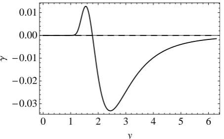
0 1 2 3 4 5 6

0.03

0.02

0.01

0.00 0.01

y

Γ

Fig. 2. Normalized growth rates of the two solutions of the disper-sion relation forβ_⊥2=0.05=5β_k2(Ap=4). Solid and dashed lines correspond to solid and dashed curves in Fig. 1, respectively.

and write a set of ordinary differential equations for all the parameters of the equilibrium distribution function, given by

dU

dτ =K1(τ ) , (11)

dβk

dτ = 1 βk(τ )

K2k(τ )−2

U (τ ) βk(τ )

K1(τ ) , (12)

dβ⊥

dτ = 1 2β⊥(τ )

K2⊥(τ ) , (13)

where τ =pt is the normalized time. Of course, at ev-ery time step, a solution of these equations will require us to solve the dispersion relation and integrate the functions Ki(τ )overk, because they depend on the parameters of the distribution function and the frequencyωk.

Finally, to close the system of equations, we use the equa-tion for the temporal evoluequa-tion of the magnetic field spectral energy per unit length (Alexandrov et al., 1984; Krall and Trivelpiece, 1986; Moya et al., 2011)

∂ε

∂τ =2γ ε , (14)

where ε=ωpp

c 1 2π L

|Bk|2

B₀2 , (15)

withLas the reference length of the plasma.

Thus, we have expressed the coupled system of Eqs. (11)– (13) as an integro-differential system, where the temporal derivatives of the parameters correspond tok-space integrals. We note that in all the equations, we have both the frequency and growth rate, thus, to solve the system we need to explic-itly solvex(y)andγ (x, y)from Eqs. (3) and (4).

2.3 Numerical results

0 200 400 600 800 1000 0.9

1.0 1.1 1.2 1.3 1.4

Τ Tp

Τ

Tp

0

T

T

Fig. 3. Temporal evolution of both proton temperatures with respect to their initial values. Solid and dashed lines correspond to perpen-dicular and parallel temperatures, respectively.

2, hence, the separation between points is dy=0.01. The origin has been avoided for obvious reasons. The time step is chosen to bedτ=0.025. Knowing the magnetic field spec-trum and the value of the parameters at a timeτ we can solve the dispersion relation to obtainxandγ, as a function ofy, at this particular time. Then, we can calculate the integrals defined in the system of equations (Eqs. 11–14), to evaluate the time derivative of each parameter. So, with that informa-tion, we use a 4th order Runge-Kutta method (Garc´ıa, 2000) to evolve the whole system to the next time stepτ+dτ. Nu-merical integration is performed fromτ=0 untilτ=1000 using the Alfv´en branch (solid line in Fig. 1). As initial val-ues we use the same valval-ues ofUpandβjused in Figs. 1 and 2, and we choose a Gaussian initial magnetic field spectrum ε(t=0)=0.35e−5y2 , −2π < y <2π . (16) The range iny-space was chosen in order to compare with the results of the hybrid simulations shown in the next sec-tion. The Gaussian profile (Eq. 16) of the initial magnetic energy spectrum was chosen to concentrate most of the wave energy in low frequency waves, with negligible power for y >1 (hence x <1), e.g., below the proton resonance fre-quency as has been observed in the solar wind (Cranmer et al., 1999a,b). Even though the free energy is equally par-titioned between waves and particles (Moya et al., 2011), it still has a non-negligible amount of the free energy in the γ >0 region as in Yoon (1992).

Due to the shape ofγ (x, y)of the solid curve in Fig. 2, only a small portion of the initial waves will effectively in-teract with the particles. Furthermore, due to the shape of K1(τ )in Eq. (11), in every time step the total time deriva-tive ofU is essentially zero, so that the proton drift speed can be considered essentially a constant. This is due to the fact that the contribution of the wave momentum to the total momentum is of the order of(VAp/c)21. Thus, for low frequency waves, in this approximation, there is no transfer of momentum between particles and waves.

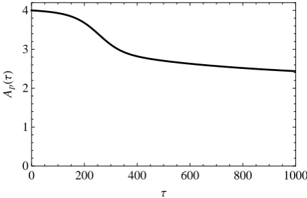
0 200 400 600 800 1000

0 1 2 3 4

Τ Ap

Τ

Fig. 4. Proton thermal anisotropy in the quasilinear solution.

It is important to mention that in the quasilinear approxi-mation, the whole temporal dependence of the macroscopic parameters of the distribution function depend strongly on the imaginary part of the frequency. In the case of the chosen parametersγ ∼10−2, thus integrating untilt∼103 is long enough to observe significant quasilinear effects, but not to consider higher order nonlinear effects, such as mode cou-pling, etc.

The temporal evolution of the two temperatures of the pro-tons, with respect to their initial values, is shown in Fig. 3. We see evidence of a parallel heating (dashed curve in Fig. 3) and a perpendicular cooling (solid curve in Fig. 3) of the plasma. For large times the heating saturates and it seems that the system is slowly approaching a metastable situa-tion whereTk6=T⊥. At the end of the integrated interval,

τ=1000, the parallel temperature Tk isTk∼1.4Tk(0)and

the perpendicular temperatureT⊥exhibits a small cooling of

no more than 5 %. Thereby, owing to the changes in both temperatures, the anisotropy also evolves as time goes on, as shown in Fig. 4. As time progresses, Ap(τ ) decreases but, due to the slowness of the process, beyondτ∼1000 it is not possible to draw conclusions about the complete behavior of the anisotropy for longer times. Towards the end of the nu-merical integration,Apdecays to a final value ofAp∼2.5.

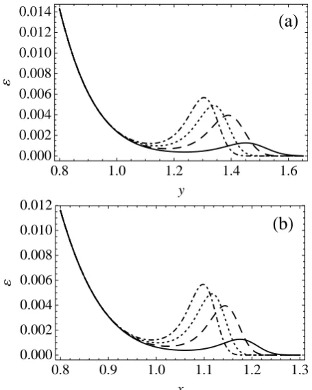
electron-proton plasma is the generation of instabilities for 1< y <1.6 (0.9< x <1.3). In Fig. 5 it is shown that the particle energy loss is transfered to the electromagnetic field as an emergence of wave modes of higher energy density than the initial ones. Thus, for the initial set of parameters in this quasilinear approximation, the whole system evolves by transferring energy from the particles to the waves, slowly approaching a metastable equilibrium.

3 Hybrid model

Due to the large difference in mass between electrons and protons, an efficient, and very common way to model a plasma system is to consider electrons as a massless fluid. Thus, we can consider protons as kinetic particles with a cer-tain velocity distribution function and electrons as a charged fluid with bulk velocityUe. As a fluid, the temporal evolution forUeis given by the momentum equation

mene dUe

dt = −ene

E+Ue c ×B

− ∇Pe, (17)

whereme is the electron mass andPe=nekBTeis the pres-sure of the electron fluid. Here, Te is the electron temper-ature and we have assumed the quasi-neutrality condition ne≈np≈n, wherenis the average density of the plasma.

In addition to the evolution of particles, we are also in-terested in following the space and time evolution of the electromagnetic field. This temporal evolution is given by Maxwell’s equations:

∇ ·B=0, ∇ ·E=4πρ , (18)

∂B

∂t = −c∇ ×E, ∂E

∂t =c∇ ×B−4πJ, (19) whereρandJ are the charge and current densities, respec-tively. Since we are interested in low frequency waves, it can be shown that the displacement current term in Ampere’s equation is of order O((VAp/c)2)and it can be neglected. Thus, we can deduce an expression for the current in terms of the curl of the magnetic field

J= c

4π∇ ×B. (20)

Similarly, the current density of a plasma with electrons and ions is given by the vectorial sum of proton and electron cur-rentsJ=en(Up−Ue). Here,Upis the fluid bulk velocity of protons. Thus, neglecting the LHS of Eq. (17), solving the equation forE, and using Maxwell’s equations (Eqs. 19), we obtain a set of equations for the hybrid model:

dxi

dt =vi, (21)

dvi dt =

e mp

E+vi c ×B

, (22)

0.8 1.0 1.2 1.4 1.6 0.000

0.002 0.004 0.006 0.008 0.010 0.012 0.014

y

a

0.8 0.9 1.0 1.1 1.2 1.3 0.000

0.002 0.004 0.006 0.008 0.010 0.012

x

b

Fig. 5. Normalized magnetic field energy spectrumεforτ=250

(solid), τ=500 (dashed), τ=750 (dotted) and τ=1000 (dot dashed). It is observed that as time advances, there is an emergence of waves at higher modes than what was originally available. (a)ε as a function of the wave numbery. (b)εas a function of the fre-quencyx.

E= −1

cUp×B+ 1

4π en(∇ ×B)×B− kBTe

en ∇n , (23)

∂B

∂t = ∇ × Up×B

₋ c

4π en∇ ×[(∇ ×B)×B], (24) wherex_i andv_i are the position and velocity of thei-th pro-ton and, in this approximation, electron temperature Te re-mains constant and equal to zero.

3.1 Hybrid expanding box model

coordinatesx , y , z at a constant velocityU0xˆ (Velli et al., 1990; Grappin and Velli, 1996; Liewer et al., 2001). The ra-dial position of the box, relative to the origin ofSis given by R=R(t )=R0+U0t, whereR0xˆ is the position of the box att=0. Then, to transform coordinates to a frame moving with the box (theS0 frame with coordinatesx0, y0, z0) a two step transformation process is done. First, a Galilean shift betweenxandx0, and then a stretching inyandz. Namely,

x=x0+R , (25)

y=ay0, (26)

z=az0, (27)

wherea=1+U0t /R0.

These transformations imply that, for an observer moving within the box, the box does not change its volume, but for an observer at rest with respect to theSframe, the box is ex-panding as it moves away from the origin. Then, using these transformations (25)–(27) it is possible to represent the time and the spatial derivatives in theS0 frame, and then to ex-press Eqs. (21)–(24) for the hybrid model in the expanding box frame (Liewer et al., 2001) as

dx0_i

dt =A(t )·v

0

i, (28)

dvi

dt = dv_i0

dt0 +

U0

R0

P·v0_i, (29)

E0= −1 cU

0 p×B

0₊ 1 4π en ∇

0_×B0

×B0−kBTe

en ∇n , (30) ∂B0

∂t0 +B 0

(∇0·U0_p)−(B· ∇0)U0_p+(U0_p· ∇0)B0

+ c

4π en∇

0_×

∇0×B0

×B0

= −U0 R L·B

0

, (31)

where the0quantities are measured in the moving frame. The derivative operators are given by

∇0= ˆx ∂ ∂x0+ ˆy

1 a

∂ ∂y0+ ˆz

1 a

∂ ∂z0 ,

∂ ∂t ≡

∂

∂t0−U0·∇ 0

, (32) and P=diag(0,1,1),L=diag(2,1,1) and A(t )= diag(1,1/a,1/a) are diagonal matrices. Also, a can be written asa=1+τ, whereτ is the time normalized to the proton cyclotron frequencyp, and=U0/(R0p). 3.2 Numerical results

As a first approximation to the problem, and to compare with the quasilinear results, we have performed a standard numer-ical hybrid simulation in one spatial dimension (thex coordi-nate) and three dimensions in velocity space, in the presence of a background magnetic fieldB0=B0xˆ. To solve the fields

equation, we use a periodic system inx, withNx=512 cells of sizedx=0.5 and 1000 particles per cell, where we have chosen the same spatial normalization as in the quasilinear case, namely the ion inertial lengthλp=VAp/ p. The par-ticle and field equations are integrated in time using a ratio-nal Runge-Kutta method (Ofman et al., 2001, 2011), whereas the spatial derivatives are calculated using a pseudo-spectral fast Fourier transform method. The time step used wasdτ = 0.025 and the simulation was performed untilτ=1000.

In the case of standard hybrid simulations, the natural choice for a reference frame is the electron frame. Thus, to keep quasi-neutrality and parallel zero current, the initial condition for proton drift isU=0. The velocity distribution function is initialized as a bi-Maxwellian using a random number generator and, in order to compare the quasilinear and hybrid models, we choose the same initial values for both proton temperaturesβ_⊥2=0.05=5β_k2 andTe=0 for elec-trons. The parallelxcomponent of the magnetic field remains constant, equal toB0, throughout the simulations. For the ini-tial parameters mentioned, we have performed simulations with an initial Gaussian perpendicular magnetic field with random phases, where, in order to compare, the amplitude and exponent of the Gaussian was chosen to have the same magnetic spectrum as in the quasilinear method (Eq. 16).

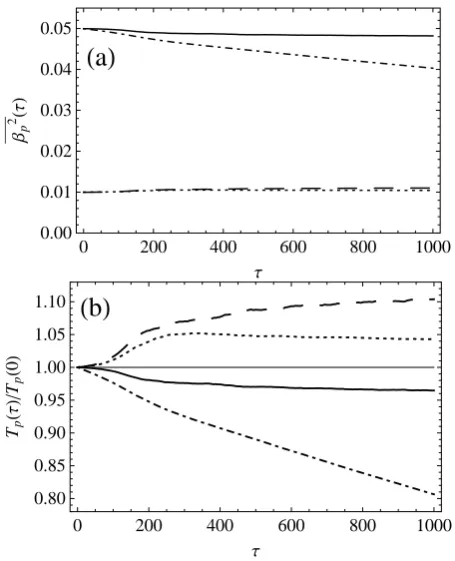
In Fig. 6a, we show the time dependence of perpendicu-lar and parallel temperatures during the simulation for the hybrid models. Comparing with the quasilinear method, the figure shows that in the case of the standard hybrid simula-tion, parallel heating (dashed curve in Fig. 6) is slower, and perpendicular cooling (solid curve in the figure) is similar to the quasilinear solution, due to the fully nonlinear res-onant absorption present in hybrid models. Thus, as it can be seen in Fig. 6b, the final values obtained correspond to T⊥∼0.95T⊥(0) and Tk∼1.1Tk(0) for perpendicular and

parallel temperatures, respectively. However, the combined effects produce a final, nonzero value (Ap∼3.4) of the ther-mal anisotropy. Compared to the quasilinear case, as shown in Fig. 7, it is observed that, although the time evolution of both curves does not match, the slopes of both curves are similar. Thus, qualitatively the two approaches agree. Also, like in the quasilinear approach, in our simulations the fluid driftUhad no significant changes. It is important to mention that it is expected that both models differ. In the quasilinear approach, we follow just one solution (the Alfv´en branch) of the dispersion relation and the nonlinear terms are approxi-mated by the quasilinear theory. On the other hand, in hybrid models, the simulations consider all the branches of the dis-persion relation, including the instabilities propagating anti-parallel to the background magnetic field. Also, being com-pletely nonlinear, hybrid simulations include several nonlin-ear effects as coupling (wave-wave interaction) between all the modes allowed by the dispersion relation.

0 200 400 600 800 1000 0.00

0.01 0.02 0.03 0.04 0.05

Τ Βp

2 Τ

a

0 200 400 600 800 1000

0.80 0.85 0.90 0.95 1.00 1.05 1.10

Τ Tp

Τ

Tp

0

b

Fig. 6. (a) Normalized proton temperatures as a function of time for both hybrid simulations (with and without expansion). Dotted and dot-dashed curves correspond to parallel and perpendicular temper-atures in the expanding box model simulation (with=10−4), re-spectively. On the other hand, dashed and solid curves correspond to parallel and perpendicular temperatures for simple hybrid simu-lations (=0). (b) The same evolution shown in panel (a), but with respect to the initial values of both temperatures for the simple and expanding box simulations.

there are no significant differences between both models in the time dependence of parallel temperatures (dashed and dotted curves in Fig. 6a), the expansion hastens the decline in this quantity as time evolves in the case of perpendicu-lar temperature (dot-dashed curve). Also, in Fig. 6b we show both temperatures with respect to their initial values. The fig-ure shows that parallel temperatfig-ure increases by 5 % while the perpendicular temperature decreases approximately to a value ofT⊥∼0.8T⊥(0). Thus, the thermal anisotropy in the

expansion model relaxes faster than in the standard model without expansion, as it can be seen in Fig. 7, reaching a value ofAp(τ=1000)∼2.9. Also, as the expansion is reg-ulated bya(τ )=1+τ (in our simulations we chose = 10−4) from the figure it is clear that notable effects only oc-cur at long enough timesτ∼200. It is important to mention that in the case of the solar corona and solar wind, that corre-spond to spherically expanding plasmas,∼10−5. However, if we can see qualitative differences between the simple and the expanding box hybrid models at times of orderτ ∼103 we need to amplify theparameter to be able to draw

con-0 200 400 600 800 1000

1.0 1.5 2.0 2.5 3.0 3.5 4.0

Τ

Ap

Τ

Fig. 7. Proton thermal anisotropy for standard=0 (solid) and

ex-panding box=10−4(dashed) hybrid simulations. Here it can be seen that the expansion effects are notable only from long enough times during the simulation. In order to compare, the anisotropy for the quasilinear solution is also included (dotted curve).

0 200 400 600 800 1000

0.000 0.005 0.010 0.015

Τ

By 2

Bz

2

Fig. 8. Temporal evolution of the perpendicular magnetic field en-ergy in simple (solid) and expanding box (dashed) hybrid models. Note that significant effects appear only afterτ∼200 as in the case of thermal anisotropy.

clusions about the differences and similarities between both methods (Liewer et al., 2001).

4 Discussion and conclusions

Starting from two different kinetic approaches, the first the-oretical based on quasilinear theory and the second based on computational simulations of hybrid models, we have done numerical studies on the interaction of waves and protons.

For the chosen parameters, our results indicate that, due to the shape of theKjfunctions in our quasilinear method, the main change occured in the parallel temperature, while in the case of the hybrid code without expansion, the main effect of the interaction between particles and waves was a decrease of the perpendicular temperatures. However, the quasilinear and the standard hybrid simulations agree on the macroscopic evolution of the drift velocity parallel to the ambient mag-netic field, and also agree on the evolution of the slope of the thermal anisotropy, even when both approaches differ in the absolute time profile of the temperatures and anisotropies.

We also performed numerical simulations using an ex-panding box hybrid model using the same initial parameters as in the quasilinear and standard hybrid models. Our results show how the expansion produces a relaxation of the system in the perpendicular plane. This model shows a decrease of the average magnetic field energy and also the typical cool-ing of an expandcool-ing gas. Nevertheless, due to thea=1+τ parameter, those effects are significant only for long enough times.

In conclusion, our results allow us to obtain and compare the basic properties of the wave-particle interaction, in sim-ple electron-proton plasmas, using different models. Numer-ical results show that both quasilinear and nonlinear meth-ods qualitatively agree in the evolution of the macroscopic plasma parameters, and this seems to suggest that resonant absorption and the energy cascade mentioned above may be relevant in the heating of solar wind plasma.

Acknowledgements. Pablo S. Moya is grateful to Comisi´on Na-cional de Ciencia y Tecnolog´ıa (CONICyT, Chile) Doctoral Fel-lowship D-21070397 and CONICyT/Becas-Chile felFel-lowship for doctoral internship at NASA/GSFC at 2010. We also acknowl-edge support from FONDECyT grants No1080658, No. 1110135, No. 1110729 and No. 1121144.

Editor-in-Chief M. Pinnock and Topical Editor R. Forsyth thank P. Yoon and one anonymous referee for their help in evaluating this paper.

References

Alexandrov, A. F., Bogdankevich, L. S., and Rukhadze, A. A.: Prin-ciples of Plasma Electrodynamics, Springer-Verlag, Berlin Hei-delberg, 1984.

Araneda, J. A., Vi˜nas, A. F., and Astudillo, H.: Proton core temper-ature effects on the relative drift and anisotropy evolution of the ion beam instability in the fast solar wind, J. Geophys. Res., 107, 1453, doi:10.1029/2002JA009337, 2002.

Aschwanden, M. J.: Physics of the Solar Corona. An Introduction with Problems and Solutions, Praxis Publishing Ltd., 2006. Astudillo, H. F.: High-order modes of left-handed electromagnetic

waves in a solar-wind-like plasma, J. Geophys. Res., 101, 24433– 24442, 1996.

Axford, W. I. and McKenzie, J. F.: The origin of the high speed solar wind streams, University Press, New York, 1992.

Axford, W. I. and McKenzie, J. F.: Acceleration of the solar Wind, in: Solar Wind Eight, AIP Conf. Proc., p. 382, Pergamon, New York, 1996.

Bale, S. D., Kellog, P. J., Mozer, F. S., Horbury, T. S., and Reme, H.: Measurement of the Electric Fluctuation Spectrum of Mag-netohydrodynamic Turbulence, Phys. Rev. Lett., 94, 215002, doi:10.1103/PhysRevLett.94.215002, 2005.

Bale, S. D., Kasper, J. C., Howes, G. G., Quataert, E., Salem, C., and Sundkvist, D.: Magnetic Fluctuation Power Near Proton Temper-ature Anisotropy Instability Thresholds in the Solar Wind, Phys. Rev. Lett., 103, 211101, doi:10.1103/PhysRevLett.103.211101, 2009.

Birdsall, C. K. and Langdon, A. B.: Plasma Physics via Computer Simulations, McGraw-Hill Company, 1985.

Cranmer, S. R.: Coronal holes and the high-speed solar wind, Space Sci. Rev., 101, 229–294, 2002.

Cranmer, S. R.: New insights into solar wind physics from SOHO, in: 13th Cambridge Workshop on Cool Stars, Stellar Systems and the Sun, edited by: Favata, F., Hussain, G. A. J., and Battrick, B., vol. 560 of ESA Special Publication, p. 299, 2005.

Cranmer, S. R., Field, G. B., and Kohl, J. L.: Spectroscopic con-straints on models of ion-cyclotron resonance heating in the po-lar sopo-lar corona an high speed sopo-lar wind, Astrophys. J., 518, 481–501, 1999a.

Cranmer, S. R., Kohl, J. L., Noci, G., Antonucci, E., Tondello, G., Huber, M. C. E., Strachan, L., Panasyuk, A. V., Gardner, L. D., Romoli, M., Fineschi, S., Dobrzycka, D., Raymond, J. C., Ni-colosi, P., Siegmund, O. H. W., Spadaro, D., Benna, C., Ciar-avella, A., Giordano, S., Habbal, S. R., Karovska, M., Li, X., Martin, R., Michels, J. G., Modigliani, A., Naletto, G., O’Neal, R. H., Pernechele, C., Poletto, G., Smith, P. L., and Suleiman, R. M.: An empirical model of a polar hole at solar minimum, Astrophys. J., 511, 481–501, 1999b.

Dasso, S., Milano, L. J., Matthaeus, W. H., and Smith, C. W.: Anisotropy in Fast and Slow Solar Wind Fluctuations, Astrophys. J., 635, L181–L184, 2005.

Davidson, R. C. and Ogden, J. M.: Electromagnetic ion cyclotron instability driven by ion energy anisotropy in high-beta plasmas, Phys. Fluids, 18, 1045–1050, 1975.

Dawson, J. M.: Particle simulation of plasmas, Rev. Mod. Phys., 55, 403–447, 1983.

Esser, R., Fineschi, S., Dobrzycka, D., Habbal, S. R., Edgar, R. J., Raymond, J. C., Kohl, J. L., and Guhathakurta, M.: Plasma prop-erties in coronal holes derived from measurements of minor ions spectral lines and polarized white light intensity, Astrophys. J. Lett., 510, L63–L67, 1999.

Fried, B. D. and Conte, S. D.: The Plasma Dispersion Function, Academic, San Diego, California, 1961.

Garc´ıa, A. L.: Numerical methods for Physics, Prentice-Hall, New Jersey, 2nd ed. edn., 2000.

Gary, P. S., Wang, J., Winske, D., and Fuselier, S. A.: Proton tem-perature anisotropy upper bound, J. Geophys. Res., 102, 27159– 27170, 1997.

Gomberoff, L. and Elgueta, R.: Resonant acceleration ofa-particles by ion-cyclotron waves in the solar wind, J. Geophys. Res., 96, 9801–9804, 1991.

Gomberoff, L. and Valdivia, J. A.: Proton-cyclotron instability in-duced by the thermal anisotropy of minor ions, J. Geophys. Res., 107, 1494, doi:10.1029/2002JA009357, 2002.

Gomberoff, L. and Valdivia, J. A.: Ion cyclotron instability due to the thermal anisotropy of drifting ion species, J. Geophys. Res., 108, 1050, doi:10.1029/2002JA009576, 2003.

Gomberoff, L., Mu˜noz, V., and Valdivia, J. A.: Ion cyclotron insta-bility triggered by drifting minor ion species: Cascade effect and exact results, Planet. Space Sci., 52, 679–684, 2004.

Grappin, R. and Velli, M.: Waves and streams in the expanding solar wind, J. Geophys. Res., 101, 425–444, 1996.

Hellinger, P. and Tr´avniˇceck, P.: Oblique proton fire hose instabil-ity in the expanding solar wind: Hybrid simulations, J. Geophys. Res., 113, A10109, doi:10.1029/2008JA013416, 2008.

Hollweg, J. V. and Isenberg, P. A.: Generation of the fast solar wind: a review with emphasis on the resonant cyclotron interaction, J. Geophys. Res., 107, 1147, doi:10.1029/2001JA000270, 2002. Horbury, T. S., Forman, M. A., and Oughton, S.: Spacecraft

ob-servations of solar wind turbulence: an over-view, Plasma Phys. Controlled Fusion, 47, B703, 2005.

Horbury, T. S., Forman, M., and Oughton, S.: Anisotropic Scal-ing of Magnetohydrodynamic Turbulence, Phys. Rev. Lett., 101, 175005, doi:10.1103/PhysRevLett.101.175005, 2008.

Hu, Y. Q. and Habbal, S. R.: Resonant acceleration and heating of solar wind ions by dispersive ion cyclotron waves, J. Geophys. Res., 104, 17045–17056, 1999.

Isenberg, P. A.: The kinetic shell model of coronal heating and ac-celeration by ion-cyclotron waves: 2. Inward and outward prop-agating waves, J. Geophys. Res., 106, 29249–29260, 2001. Isenberg, P. A. and Vasquez, B. J.: Preferential perpendicular

heat-ing of coronal hole minor ions by the Fermi mechanism, Astro-phys. J., 668, 546–556, 2007.

Kamide, Y. and Chian, A. C. L. (Eds.): Handbook of the Solar-Terrestrial Environment, Springer-Verlag, Berlin Heidelberg, 2007.

Kivelson, M. G. and Russell, C. T. (Eds.): Introduction to Space Physics, Cambridge University Press, Cambridge, 1995. Kohl, J. L., Noci, G., Antonucci, E., Tondello, G., Huber, M. C. E.,

Cranmer, S. R., Strachan, L., Panasyuk, A. V., Gardner, L. D., Romoli, M., Fineschi, S., Dobrzycka, D., Raymond, J. C., Ni-colosi, P., Siegmund, O. H. W., Spadaro, D., Benna, C., Ciar-avella, A., Giordano, S., Habbal, S. R., Karovska, M., Li, X., Martin, R., Michels, J. G., Modigliani, A., Naletto, G., O’Neal, R. H., Pernechele, C., Poletto, G., Smith, P. L., and Suleiman, R. M.: UVCS/SOHO a empirical determinations of anisotropic velocity distributions in the solar corona, Astrophys. J., 501, L127–L131, 1998.

Krall, N. A. and Trivelpiece, A. W.: Principle of Plasma Physics, San Francisco Press Inc., 1986.

Leamon, R. J., Matthaeus, W. H., Smith, C. W., Zank, G. P., Mullan, D. J., and Oughton, S.: MHD-driven Kinetic Dissipation in the Solar Wind and Corona, Astrophys. J., 537, 1054–1062, 2000.

Liewer, P. C., Velli, M., and Goldstein, B. E.: Alfv´en wave prop-agation and ion cyclotron interaction in the expanding solar wind: One-dimensional hybrid simulation, J. Geophys. Res., 106, 29261–29281, 2001.

Marsch, E.: Closure of multi-fluid and kinetic equations for cyclotron-resonant interactions of solar wind ions with Alfv´en waves, Nonlin. Processes Geophys., 5, 111–120, doi:10.5194/npg-5-111-1998, 1998.

Matsumoto, H. and Omura, Y. (Eds.): Computer Space Plasma Physics: Simulation Techniques and Software, Terra Scientific Publishing Company, Tokyo, 1993.

Matteini, L., Landi, S., Hellinger, P., and Velli, M.: Par-allel proton fire hose instability in the expanding solar wind: Hybrid simulations, J. Geophys. Res., 111, A10101, doi:10.1029/2006JA011667, 2006.

Matthaeus, W. H., Goldstein, M. L., and Roberts, D. A.: Evidence for the presence of quasitwo-dimensional nearly incompressible fluctuations in the solar wind, J. Geophys. Res., 95, 20673– 20683, 1990.

Matthaeus, W. H., Ghosh, S., Oughton, S., and Roberts, D. A.: Anisotropic three-dimensional MHD turbulence, J. Geophys. Res., 101, 7619–7630, 1996a.

Matthaeus, W. H., Zank, G. P., and Oughton, S.: Phenomenology of hydromagnetic turbulence in a uniformly expanding medium, J. Plasma Phys., 56, 659–675, 1996b.

Moya, P. S., Mu˜noz, V., Rogan, J., and Valdivia, J. A.: Study of the Cascading Effect During the Acceleration and Heating of Ions in the Solar Wind, J. Atmos. Solar-Terr. Phys., 73, 1390–1397, 2011.

Ofman, L., Vi˜nas, A., and Gary, S. P.: Constraints on theO+5 anisotropy in the solar corona, Astrophys. J., 547, L175–L178, 2001.

Ofman, L., Vi˜nas, A.-F., and Moya, P. S.: Hybrid models of solar wind plasma heating, Ann. Geophys., 29, 1071–1079, doi:10.5194/angeo-29-1071-2011, 2011.

Pavan, J., Yoon, P. H., and Umeda, T.: Quasilinear theory and simulations of Buneman instability, Phys. Plasmas, 18, 042307, doi:10.1063/1.3574359, 2011.

Smith, C. W., Matthaeus, W. H., Zank, G. P., Ness, N. F., Oughton, S., and Richardson, J. D.: Heating of the low-latitude solar wind by dissipation of turbulent magnetic fluctuations, J. Geophys. Res., 106, 8253–8272, 2001.

Smith, C. W., Isenberg, P. A., Matthaeus, W. H., and Richardson, J. D.: Turbulent Heating of the Solar Wind by Newborn Inter-stellar Pickup Protons, Astrophys. J., 638, 508–517, 2006. Tu, C. Y. and Marsch, E.: Study of the heating mechanism of the

solar wind in coronal hole, in: Solar Wind Nine, AIP Conf. Proc., p. 373, Woodbury, New York, 1999.

Velli, M., Grappin, R., and Mangeney, A.: Solar wind expansion effects on the evolution of hydromagnetic turbulence in the in-terplanetary medium, Computer Physics Communications, 59, 153–162, 1990.

Yoon, P. H.: Quasilinear evolution of Alfv´en-ion-cyclotron and mir-ror instabilities driven by ion temperature anisotropy, Phys. Flu-ids B, 4, 3627–3637, 1992.